Kalman Filter Overview

Problem Formulation

Equation (1) – (5) shows the formulation of the Kalman Filter problem. Equation (1) is the measurement model, which shows how observers get measurement variables. The measurement variable is measured from “state” which is transformed by a linear matrix F. Equation (2) shows the system model which shows how “state” is going to transition by time steps. The “state” variables are what we actually would like to know, but since the additive gaussian noise v is added and it is transformed by the linear transformation, the “state” variables vector cannot be known directly. It is so called Hidden-Gaussian Model. And also, therefore the “state” is transitioning by time steps (which is called the Markov model), and the “state” cannot be stable.

We have the other assumption on the additive noise “v” and “w”. The noise characteristics follow white gaussian noise, the average of the noise shall be 0 and the covariance matrix shall be R and Q.

\begin{align} m_t = F_ts_t + v_t \\ s_{t+1} = F_ts_t + G_tw_t \\ \quad \quad Cov(v_t) = R_t, \quad Cov(v_t) = Q_t \end{align}

Because v and w are white gaussian noise, as we can see in (4), there is no correlation. And also, since we set the initial variable for the state as gaussian, there is no correlation between x and gaussian white noise v, w.

\begin{align} E \text{\textbraceleft} \begin{bmatrix} w_t \\ v_t \end{bmatrix} \begin{bmatrix} w_s^T & v_s^T \end{bmatrix} ]\text{\textbraceright} = \begin{bmatrix} Q_T & 0 \\ 0 & R_t \end{bmatrix} \delta_{ts}, \quad R_t > 0 \\ s_0 \text{\textasciitilde} \Nu( \overline{s_0}, \Sigma_0) \\ E \text{\textbraceleft} w_tx_s^T \text{\textbraceright} = 0, \quad E \text{\textbraceleft} v_tx_s^T \text{\textbraceright} = 0 \\ \end{align}

Kalman Filter

But how we can solve this formulation? We basically use the linear transformation of the Gaussian vectors. We easily expand the formulation and get equations (7) – (11) using gaussian transformation. For using Kalman Filter, we repeat system updates and measurement updates. When we do not have measurement information and update “state” information by time step, The system updates are applied. The state is updated based on the system model and then its covariance matrix is also updated using covariance matrix Q which is from system noise w.

\begin{align} \hat{s_t}=F_ts_{t-1} \\ \hat{P_t}=FP_{t-1}^TF_t^T + G_TQ_tG_t^T \\ \end{align}

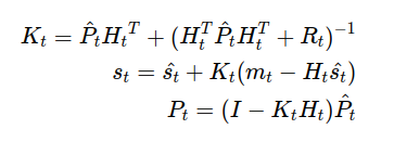
And then, when we get measurement information from sensors or something, the measurement updates are applied for the estimated “state” vector. The Kalman Gain (9) is computed to estimate the “state” and its covariance matrix.

So what do these procedures mean?

As we can see in (10), the estimated state (which is on the left side of (10)) is updated by s from (7) and the measurement values m. It means that the latest estimated “state” is determined by confidence from both gaussian variables s and m. If there is much confidence in measurement information more than that of state on the former time step, the latest state is mostly determined by measurement information. On the contrary, if there is much confidence in the system model, the “state” is going to emphasize the system model which is gotten from the former “state” variable.

Because all these formulations are solved using just linear algebra operations, it is lightweight. But we have to care about the inverse matrix in (9) for getting Kalman Gain. We cannot say Inverse matrix computations are generally stable. If we would like to use Kalman Filter with stability, we should use decomposition operations such as UD decomposition or Square decomposition operation. We can see the sort of implementation in [2]