Note: Quantum Computing (1)

Quantum Computing

O is called an observable quantity and corresponds to an observed physical quantity. A vector α expresses information about the probability distribution of measurement results and is called a quantum state. The expected value of a random variable O is expressed in the quadratic form of O and α
We express the time evolution of quantum systems in a unitary way, just as we express the time evolution in stochastic statistics as Markov processes. A unitary matrix that represents a unitary transformation has the following property that its inverse is equivalent to the complex conjugate matrix:

\begin{align} U^{-1} = U^{\dagger} \end{align}

By switching from amplitude vector descriptions to density matrices, a statistical mixed states of quantum can be incorporated into the formalism of quantum mechanics. The density matrix ρ is given by the direct product ρ=ααT and can be regarded as the covariance matrix of α.
A composite system of systems can be described by combining density matrices.
At the beginning of this book, it is described in matrix form, but in quantum mechanics, it is basically written in Dirac notation. The left side of the Dirac form is called “bra”, which indicates the complex conjugate of the vector, and the right side is called “ket”, which can be combined with “bra” to express the inner product. A description example using the Dirac form is shown below. For example,

State space

Unitary Matrix and Operator

\begin{align} U \alpha = \alpha' \\ U\ket{\psi}=\ket{\psi'} \end{align}

Hermite Matrix and Operator

\begin{align} O\isin C^{n×n} \\ O \end{align}

Some Rules of Dirac Form (Norm of a Vector Psi,,, etc)

All vectors that is satisfying (8) on the Hilbert space can be expressed as (9)

\begin{align} \begin{Vmatrix} \psi \end{Vmatrix}=\sqrt{\braket{\psi|\psi}} \\ \braket{\psi_2|\psi_1}^*=\braket{\psi_1|\psi_2} \\ \braket{e_i|e_j}=\delta_{ij} \\ \ket{e_i} = \displaystyle\sum_{i} \braket{e_i|\psi}\ket{e_i} \\ \bold{1} = \displaystyle\sum_{i} \ket{e_i}\bra{e_i} \\ \end{align}

Amplitude Vector

Amplitude Vecotr Phi means randomness of state vector that is coming from quantum behavior. If an amplitude vectors is below,emerging either states of elemnets is 50 50 chance.

\ket{\psi_i} = {1\over \sqrt{2}} (1, 1)

Density Operator Rho

By switching from amplitude vectors form to density matrices form, statistical mixed states can be incorporated into the quantum mechanical formulation. What this formula means is that it simultaneously deals with quantum randomness and the randomness of the mixed state when you know the mixed ratio of probabilities on each amplitude vectors.

You can pull subsystem out from whole system by using density matrix form. The operation that pulls subsystem out is so called “Marginalization”, and corresponding to “Trace Operation” along with “combination” of density matrix in Mathematics.

Given that the system is state phi(k=1,,,K) with probability pk, the density operator ρ describing this mixed quantum state is written as

\begin{align} \rho = \displaystyle\sum_{k=1}^Kp_k \ket{\psi_k}\bra{\psi_i} \\ p_k \ge 0 , \sum p_k = 1 \end{align}

Due to factors like external disturbances, it is difficult to maintain the state of quantum bits indefinitely.

For example, consider a superposition state of |0> and |1>, and a state where |0> and |1> are mixed with a 50% probability for each. Both of these states have an equal statistical probability of measuring |0> or |1>.

However, when measured in the Hadamard basis, the former state will always yield |+> with certainty, while the latter state will result in a 50-50 chance of measuring |+> or |->.

Observables

In quantum computing, “Observables” refer to operators used to measure the physical properties or states of a quantum system. They play a crucial role when manipulating and measuring the state of quantum bits (qubits) in quantum computing.

Observables are represented as Hermitian operators. The Hermitian operators represent physical quantities, and during measurement, they project the state of the quantum bit onto a basis state (e.g., |0> or |1>) to obtain physical information such as energy, spin, or position.

O^\dagger = O

Observables are essential concepts in quantum computing, as they are fundamental to understanding and designing quantum algorithms and calculations.

The Hermite operator O has a diagonal component representation with respect to the set of eigenvalues {oi} and the corresponding eigenvector ei.

This contains information corresponding to quantum physical quantities such as position, momentum, and spin. Each element, vector corresponds to an amplitude vector, and it is possible to calculate the expected value of an observable using the amplitude vector.

Using this spectral representation, the analytic function f (14) can be applied.

\begin{align} O = \displaystyle\sum_{i} o_i \ket{e_i}\bra{e_i} \\ f(O)=\displaystyle\sum_{i} f(o_i) \ket{e_i}\bra{e_i} \\ \end{align}

The expected value of the quantum system observation charge O can be calculated as (15).

In the case of the pure state(16), the expected value of the observables is given by (17).

\begin{align} \braket{O} = tr\lbrace\rho O\rbrace \\ \rho= \ket{\psi}\bra{\psi} \\ \braket{O} = \braket{\psi|O|\psi} \end{align}

Since the density matrix is another description of amplitude vector, the expectation of the Observable is gotten using either form. Pauli matrices are frequently used as the operator.

Utilizing Commutativity

Let observables A and B be Hermitian operators, and its eigen value and vector of A is represented as

A |a\rangle = a |a\rangle

If they are commutative, which means the following relationship.

AB=BA

In this case, A and B share the common eigenvector.

A(B |a\rangle) = \lambda (B |a\rangle)

Since A and B share the common eigenvector, its additive Hermite C has also common eigen vector.

C |a\rangle = (A + B) |a\rangle = A |a\rangle + B |a\rangle = a |a\rangle + b |a\rangle = (a + b) |a\rangle

If observables are commutative, they have a common eigenstate in which each observable can be measured individually or in combination, and the measurements do not affect each other.

Time Evolution

Time Extension of Quantum System is describled using Schrödinger equation. Where H denote the Hamiltonian, h-bar is Planck’s constant.

\begin{align} i\hbar\frac{d}{dt}\ket{\psi}=H\ket{\psi} \end{align}

The time evolution of a mixed state of quantum system described by the density operator p is written as follows. (using (11) and (18))

\begin{align} i\hbar\frac{d}{dt}\rho(t)=\frac{d}{dt}\displaystyle\sum_{i} p_i \ket{\psi_i}\bra{\psi_i} \\ = H\rho - \rho H = \lbrack H, \rho \rbrack \end{align}

Quantum Measurement

Measurement in a quantum system is to apply a projective transformation. This measurement is called a projective measurement. The oi is the result of the measurement associated with the projection Pi.

\begin{align} O=\displaystyle\sum_{i} o_iP_i \end{align}

\begin{align} p(o_i)=tr\lbrace P_n O\ket{\psi}\bra{\psi} \rbrace = \begin{Vmatrix} P_n \ket{\psi} \end{Vmatrix}^2 \\ \end{align}

The status after measurement is as follows.

\ket{\psi} \mapsto \frac{P_n\ket{\psi}}{\sqrt{\bra{\psi}P_n\ket{\psi}}}

An Example of projective measurement

When it comes to measure along with 0> and 1>, projection matrices are written in followings.

M_0=\ket{0}\bra{0}, M_1=\ket{1}\bra{1}

and, the projective measurement for 0> is

\bra{\psi}M_0\ket{\psi}= \begin{bmatrix} \alpha^* &\beta^* \end{bmatrix} \begin{bmatrix} 1 \\ 0 \end{bmatrix} \begin{bmatrix} 1 & 0 \end{bmatrix} \begin{bmatrix} \alpha \\ \beta \end{bmatrix}=\|\alpha\|^2

Basis and its Projection

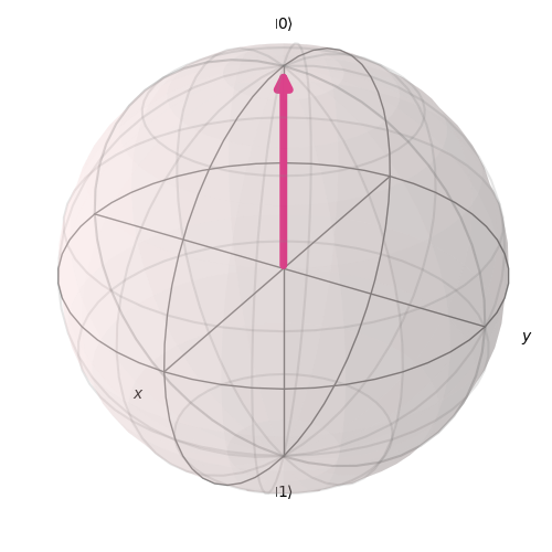
What measurement is the above projection referring to? It refers to a measurement with respect to a certain basis. There are various ways to choose the basis, such as Z basis (computational basis), X basis (Hadamard basis), and orthogonal basis on Y axis in Bloch sphere.