Classical Control Theory
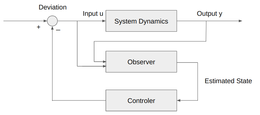
The deviation between the reference value and the output, denoted as (1), is input to the controller to determine the control input u.”
\begin{align}
e(t) = r(t) - y(t)
\end{align}
PID Control
In PID control, the control input is determined through negative feedback by applying proportional (P) control, integral (I) control, and derivative (D) control, each multiplied by respective constants, to the deviation.
\begin{align}
u(t) = - (K_py(t)+\frac{1}{T_I}\int_{0}^{t}y(\tau)d\tau+T_D\frac{dy(t)}{dt})
\end{align}
Modern Control Theory
In contrast, modern control theory utilizes state feedback, where the control input is determined by multiplying the state vector y by a matrix f.
\begin{align}
u(t) = -f^Ty(t)
\end{align}
if we use f using K or T_D, it is as same as PD control. Therefore, classical control can be viewed as an extension of modern control. However, in modern control theory, it is possible to perform more complex control by applying feedback control to n states even for systems of order n greater than 3. This allows for control of systems with higher degrees of complexity.
In modern control, systematic determination of control inputs is achieved by state estimation through observers and Kalman filters.
Model Predictive Control
Model Predictive Control (MPC) is a control strategy that uses a dynamic model of the system to predict future behavior over a finite time horizon to minimize a specified cost function. A sequence of control inputs is optimized and applied to the system. The process is repeated with updated measurements and predictions at each time step. mpc is particularly useful for systems with complex dynamics, constraints, and varying operating conditions, where control actions can be adjusted in real time to achieve desired performance.
In Model Predictive Control Theory, we employ the concept of a reference trajectory instead of an error deviation. And also, the controller computes input variations instead of control input. The input variations is described as the time difference of input u,
\begin{align}
\delta u(k) = u(k) - u(k-1)\\
\end{align}
If we use time operator z (like Z-transform),
\begin{align}
\delta u(k) = (1 - z^{-1})u(k)\\
u(k) = \frac{1}{1 - z^{-1}} \delta u(k) \\
\end{align}
At time k, the control objective for the output y is set to the reference value s. However, in Model Predictive Control (MPC), instead of directly making y track s, the output is made to follow a trajectory called the reference trajectory, denoted as r. Here, r(k+l | k) represents the reference trajectory at time k+l given the information at time k. This approach formulates the idea of adjusting the speed at which the output approaches the target value using the reference trajectory.
\begin{align}
y(k) \rightarrow s(k) \\
\epsilon(k) = s(k) - y(k) \\
\epsilon(k+l) = e^{-lT_s/T_{ref}}\epsilon(k) = \lambda^l \epsilon(k) \\
\lambda = e^{-lT_s/T_{ref}}, 0<\lambda^l<1 \\
r(k+l | k) = s(k+l) - \epsilon(k+l) = s(k+l) - \lambda^l \epsilon(k)
\end{align}
Ts represents the sampling period, and Tref represents the time constant.
Introduction of a reference trajectory is convenient, as it enables the use of purification source constraints in design to prevent excessive amplification of input signal disturbances.
In Model Predictive Control , the control inputs are determined by utilizing the predicted output values of the controlled system within a finite interval known as the prediction horizon. However, it’s evident that predicting future output values becomes difficult as they inherently depend on future control inputs. To address this, MPC establishes the prediction horizon by introducing certain assumptions about the inputs, thus influencing the subsequent predictions of future outputs.
\begin{align}
\hat{y}(k+l | k) , l = 1,2,3,,,H_p\\
\end{align}
The input, “u,” is assumed to take different values for the initial few steps of the prediction horizon and then remain constant thereafter. The range over which these distinct values are taken is referred to as the control horizon.
In essence, the process involves predicting the future responses several steps ahead at each time instant and iteratively determining the optimal input. The optimal input is often formulated as a constrained quadratic optimization problem(convex optimaization), and this formulation can be efficiently computed using solvers, facilitating rapid computations.