Image Domain Adaptation using OptimalTransport using POT library

POT library and its examples

Optimal Transport is one promising algorithm for handling data distributions. It provides a different metric compared to measures like Kullback-Leibler divergence or entropy that have been used in the past. As previously discussed in this article(https://eye.kohei-kevin.com/2023/06/22/the-concept-of-optimal-transport/), Optimal Transport allows for a comparison of data distributions that aligns with human intuition since it doesn’t directly compare densities. POT (Python Optimal Transport) is a library dedicated to dealing with Optimal Transport, and it encompasses numerous use cases. In this article, we’ve explored one of those cases.

POT page is here (https://pythonot.github.io/index.html)

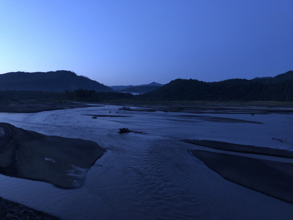
Input Images

Result

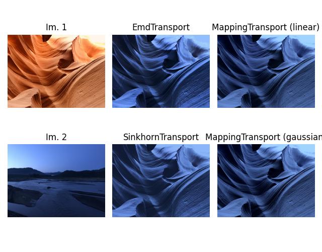
Now we got a picture of Antelope Canyon early in the morning

Code

# Authors: Remi Flamary <remi.flamary@unice.fr>
#          Stanislas Chambon <stan.chambon@gmail.com>
#
# License: MIT License

# sphinx_gallery_thumbnail_number = 3
import os
from pathlib import Path

import numpy as np
from matplotlib import pyplot as plt
import ot

rng = np.random.RandomState(42)


def im2mat(img):
    """Converts and image to matrix (one pixel per line)"""
    return img.reshape((img.shape[0] * img.shape[1], img.shape[2]))


def mat2im(X, shape):
    """Converts back a matrix to an image"""
    return X.reshape(shape)


def minmax(img):
    return np.clip(img, 0, 1)




def main(
    image1_path: str,
    image2_path: str,
    export_path: str
):

    # Loading images
    this_file = os.path.realpath('__file__')
    data_path = os.path.join(Path(this_file).parent.parent.parent, 'data')

    I1 = plt.imread(image1_path).astype(np.float64) / 256
    I2 = plt.imread(image2_path).astype(np.float64) / 256

    X1 = im2mat(I1)
    X2 = im2mat(I2)

    # training samples
    nb = 500
    idx1 = rng.randint(X1.shape[0], size=(nb,))
    idx2 = rng.randint(X2.shape[0], size=(nb,))

    Xs = X1[idx1, :]
    Xt = X2[idx2, :]

    # EMDTransport
    ot_emd = ot.da.EMDTransport()
    ot_emd.fit(Xs=Xs, Xt=Xt)
    transp_Xs_emd = ot_emd.transform(Xs=X1)
    Image_emd = minmax(mat2im(transp_Xs_emd, I1.shape))

    # SinkhornTransport
    ot_sinkhorn = ot.da.SinkhornTransport(reg_e=1e-1)
    ot_sinkhorn.fit(Xs=Xs, Xt=Xt)
    transp_Xs_sinkhorn = ot_sinkhorn.transform(Xs=X1)
    Image_sinkhorn = minmax(mat2im(transp_Xs_sinkhorn, I1.shape))

    ot_mapping_linear = ot.da.MappingTransport(
        mu=1e0, eta=1e-8, bias=True, max_iter=20, verbose=True)
    ot_mapping_linear.fit(Xs=Xs, Xt=Xt)

    X1tl = ot_mapping_linear.transform(Xs=X1)
    Image_mapping_linear = minmax(mat2im(X1tl, I1.shape))

    ot_mapping_gaussian = ot.da.MappingTransport(
        mu=1e0, eta=1e-2, sigma=1, bias=False, max_iter=10, verbose=True)
    ot_mapping_gaussian.fit(Xs=Xs, Xt=Xt)

    X1tn = ot_mapping_gaussian.transform(Xs=X1)  # use the estimated mapping
    Image_mapping_gaussian = minmax(mat2im(X1tn, I1.shape))

    #plot org

    plt.figure(1, figsize=(6.4, 3))
    plt.subplot(1, 2, 1)
    plt.imshow(I1)
    plt.axis('off')
    plt.title('Image 1')

    plt.subplot(1, 2, 2)
    plt.imshow(I2)
    plt.axis('off')
    plt.title('Image 2')
    plt.tight_layout()

    # plt.savefig(export_path)


    plt.figure(2, figsize=(6.4, 5))
    plt.subplot(1, 2, 1)
    plt.scatter(Xs[:, 0], Xs[:, 2], c=Xs)
    plt.axis([0, 1, 0, 1])
    plt.xlabel('Red')
    plt.ylabel('Blue')
    plt.title('Image 1')

    plt.subplot(1, 2, 2)
    plt.scatter(Xt[:, 0], Xt[:, 2], c=Xt)
    plt.axis([0, 1, 0, 1])
    plt.xlabel('Red')
    plt.ylabel('Blue')
    plt.title('Image 2')
    plt.tight_layout()

    plt.figure(2, figsize=(10, 5))

    plt.subplot(2, 3, 1)
    plt.imshow(I1)
    plt.axis('off')
    plt.title('Im. 1')

    plt.subplot(2, 3, 4)
    plt.imshow(I2)
    plt.axis('off')
    plt.title('Im. 2')

    plt.subplot(2, 3, 2)
    plt.imshow(Image_emd)
    plt.axis('off')
    plt.title('EmdTransport')

    plt.subplot(2, 3, 5)
    plt.imshow(Image_sinkhorn)
    plt.axis('off')
    plt.title('SinkhornTransport')

    plt.subplot(2, 3, 3)
    plt.imshow(Image_mapping_linear)
    plt.axis('off')
    plt.title('MappingTransport (linear)')

    plt.subplot(2, 3, 6)
    plt.imshow(Image_mapping_gaussian)
    plt.axis('off')
    plt.title('MappingTransport (gaussian)')
    plt.tight_layout()

    plt.savefig(export_path)


if __name__ == '__main__':

    import argparse

    parser = argparse.ArgumentParser(
        description='Domain Adaptation using Optimal Transport using POT example.'
    )
    parser.add_argument(
        '--image1_path', '-P1', type=str, default='./image/antelope.jpg', help='path for image1'
    )
    parser.add_argument(
        '--image2_path', '-P2', type=str, default='./image/early_morning.jpg', help='path for image2'
    )
    parser.add_argument(
        '--export_path', '-EP', type=str, default='./image/result.jpg', help='path for image2'
    )
    args = parser.parse_args()

    main(
        args.image1_path,
        args.image2_path,
        args.export_path
    )