Note : General Solution of Homogeneous Equation

Homogeneous Equation

The general form of homogeneous equation is written as

\begin{align}
\frac{dy}{dt} = Ay
\end{align}

If the matrix a is represented as N x N square matrix, It corresponds to N dimensional differential equations. Next, consider the approximate solution of y under the initial conditions. First, integrate the above equation (1) as the 0-th to n-th order approximation solution.

\begin{align}
y(t)=y(0)+Aty_0 \\
y(t)=y(0)+Aty_0 +A^2t^2y_0 \\
y(t)=y(0)+Aty_0 +\frac{1}{2!}A^2t^2y_0 + \cdot\cdot\cdot+ \frac{1}{n!}A^nt^ny_0
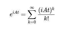
\end{align}

Although detailed description is omitted, it is shown that this series expansion converges to a certain constant and is a Taylor expansion. And also, what important here is that this series expansion is written as matrix exponential like below.

\begin{align}
y(t)=(E+At +\frac{1}{2!}A^2t^2 + \cdot\cdot\cdot + \frac{1}{n!}A^nt^n+)y_0\\
y(t)=e^{At}y_0
\end{align}

So considering and understanding this matrix exponential must be known (https://eye.kohei-kevin.com/2023/12/21/how-to-estimate-eigen-values-of-any-matrix/).

e^{A} = \sum_{k=0}^{\infty} \frac{A^k}{k!} \\
\frac{d}{dt}(e^{At})=A\frac{d}{dt}(e^{At}) \\
e^{-At}=(e^{At})^{-1} \\
e^{A (k+l)}=e^{A k} e^{Al} \\

On top of that, the matrix A can be decomposed like below If the Jordan Normal form (or digonalization) is used

A^n=(PJP^{-1})^n=PJ^nP^{-1}

So, the general solution (6) is expanded to

y(t)=e^{tA}\mathbf{c}=Pe^{tJ}P^{-1}\mathbf{c}

This looks quite beautiful, but we can use another form, using eigen values and vectors.

y(t)=\sum_{k=1}^{n}{c_ke^{\lambda_kt}u_k}\\
\lambda_k:Eigen\,Value \\
u_k:Eigen\,Vector

When it comes to Inhomogeneous Equation, Laplace Transform should be introduced. I will write down about that in the future.

An example of 2nd-order differential equation

Formulation

Let’s say there is a 2nd order differential equation below,

\frac{d^2x}{dt^2}+p\frac{dx}{dt}+q=0\\

and then, consider state vector s in state space by decomposing “x”

\begin{align}
s_1(t) = x(t), \quad s_2(t) = \frac{dx}{dt}\\
\frac{ds_1}{dt}=s_2\\
\frac{ds_2}{dt}=-qs_1 - p s_2\\
s=\begin{pmatrix}
    s_1  \\
    s_2
\end{pmatrix}\\
A=\begin{pmatrix}
    0 & 1  \\
    -q & -p
\end{pmatrix}\\
\frac{d}{dt}s=As
\end{align}

What important here is that a solution of x is represented as linear combination of state s.

x=C_1 s_1(t)+C_2 s_2(t)

In the case of a certain 2nd-order differential equation (12), (10) and (11) is represented as

\begin{align}
\frac{d^2x}{dt^2}-5\frac{dx}{dt}+6=0\\
A=\begin{pmatrix}
    0 & 1  \\
    -6 & 5
\end{pmatrix}
\end{align}

And also, if A is regular matrix, there are eigen values and vectors that satisfy following

\begin{align}
A\alpha_1=\lambda_1\alpha_1\\
A\alpha_2=\lambda_2\alpha_2\\
det(A - \lambda E)=\lambda^2+p\lambda+q=0
\end{align}

in the case of (12), eigen values are 2 and 3.

Given the eigenvalues ( \lambda_1 = 2 ) and ( \lambda_2 = 3 ), the corresponding eigenvectors can be found by solving the homogeneous equations ( (A – \lambda_i I) \mathbf{v}_i = 0 ) for ( i = 1, 2 ). The solutions to these equations provide the eigenvectors that span the solution space for the differential equation.

For \lambda_1 = 2,

(A - 2I) \mathbf{v}_1 = \begin{bmatrix} -2 & 1 \\ -6 & 3 \end{bmatrix} \mathbf{v}_1 = 0

For \lambda_2 = 3

(A - 3I) \mathbf{v}_2 = \begin{bmatrix} -3 & 1 \\ -6 & 2 \end{bmatrix} \mathbf{v}_2 = 0

\text{Solving this, we find that }\\
\mathbf{v}_1  \text{ is proportional to } \begin{bmatrix} 1 \\ 2 \end{bmatrix}\\
\mathbf{v}_2  \text{ is proportional to } \begin{bmatrix} 1 \\ 3 \end{bmatrix}

Thus, the general solution x(t) to the differential equation can be expressed as a linear combination of the modes corresponding to these eigen values:

s(t) = C_1 e^{2t}\begin{bmatrix} 1 \\ 2 \end{bmatrix} + C_2 e^{3t}\begin{bmatrix} 1 \\ 3 \end{bmatrix}\\
= \begin{bmatrix} C_1 e^{2t} + C_2 e^{3t} \\ 2C_1 e^{2t} + 3C_2 e^{3t} \end{bmatrix}=\begin{bmatrix} x(t) \\ \frac{d}{dt}x(t) \end{bmatrix}

where C_1 and C_2 are constants determined by the initial conditions of the problem.

The importance of finding the eigenvalues and eigenvectors in this context lies in their ability to decompose the solution into simpler, exponential functions which are easier to analyze and interpret. This decomposition also simplifies the solution’s behavior analysis, particularly its stability and long-term trends, as each term in the solution grows or decays exponentially according to its eigenvalue.