About
To optimize parameters, estimating gradients is quite important. Since the optimization is highly depending on gradient descent methods. In this article , I post an note that is about estimating gradients of variational quantum circuit.
Reference
https://pennylane.ai/qml/glossary/parameter_shift/
https://arxiv.org/abs/1803.00745
https://arxiv.org/abs/1811.11184
Variational Quantum Circuit
In the context of quantum computing, variational quantum circuits frequently come up. These are circuits designed to calculate the expected value of complex quantum states that have been transformed by a quantum circuit. The circuit parameters are adjusted to yield the desired output by the user. This type of circuit also seems to be applied in quantum machine learning. In classical machine learning, particularly in neural networks, how is it done? It’s done through backpropagation. We calculate the partial derivatives of the parameters based on the difference between the output and the prediction and through algebraic calculations. Such processes are crucial in optimization problems. However, how is this implemented in variational circuits? There was an explanation in a quantum computing library called PennyLane, so I will briefly summarize it.
Parameter-Shift Rule
Intunitive Explanation
They say that this is similar to how the derivative of the function sin(x).
f(x) = \sin(x) \text{ is identical to } \\
\frac{1}{2}\sin\left(x + \frac{\pi}{2}\right) - \frac{1}{2}\sin\left(x - \frac{\pi}{2}\right)
So the same scheme is used to compute both sin(x) and its derivative (at x±π/2).
Overview
Let’s say we have sequence of Unitary Gates, it compose a variational quantum circuit.
\begin{align}
U(x; \theta) = U_N(\theta_N) U_{N-1}(\theta_{N-1}) \cdots U_i(\theta_i) \cdots U_1(\theta_1) U_0(x).
 \\
U_j(\gamma_j) = \exp(i \gamma_j H_j)
\end{align}
Just looking at a parameter and its unitary gate, it is also represented like
f(x; \theta_i) = \langle 0 | U_0^\dagger(x) U_i^\dagger(\theta_i)\^B U_i(\theta_i) U_0(x) | 0 \rangle \\= \langle x | U_i^\dagger(\theta_i)\^B U_i(\theta_i) | x \rangle = \langle x | M_{\theta_i}(\hat{B})| x \rangleso we can get its gradient by
\begin{align}
\nabla_{\theta_i} f(x; \theta_i) = \langle x | \nabla_{\theta_i} M_{\theta_i}(\hat{B}) | x \rangle \in \mathbb{R} \\
\text{where } \nabla_{\theta_i} M_{\theta_i}(\hat{B}) = c \left[ M_{\theta_i + s}(\hat{B}) - M_{\theta_i - s}(\hat{B}) \right]
\end{align}
where the multiplier c and the shift s are determined completely by the type of transformation M and independent of the value of θ.
In a specific case, pauli gate
When pauli gate is used in the circuit,
U_i(\theta_i) = \exp\left(-i \frac{\theta_i}{2} \hat{P}_i\right),The gradient of the parameter (4) is represented as
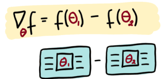
\nabla_{\theta} f(x; \theta) = \frac{1}{2} \left[ f(x; \theta + \frac{\pi}{2}) - f(x; \theta - \frac{\pi}{2}) \right]Yeah, the form is completely as same as shown before.