Finite Element Analysis using Condensation

Introduction

There is a very useful Python library for solving Finite Element Analysis (FEA) problems: Scikit-FEM.
It is much more elegant and flexible than I initially expected.
Here, I introduce a simple test case and briefly explain the background theory.

Structural Analysis with FEA

Theory – Static Condensation

One of the most stable and widely used techniques to reduce the size of an FEA system is static condensation.
Static condensation eliminates internal degrees of freedom (DOFs) so that the remaining system becomes smaller while still preserving the correct solution on the boundary DOFs.

Suppose the equilibrium equation is partitioned as follows:

\begin{align}
\begin{bmatrix}
   K_{ff} & K_{fb} \\
   K_{bf} & K_{bb}
   \end{bmatrix}
   \begin{bmatrix}
   U_{f} \\
   U_{b}
   \end{bmatrix}
   =
   \begin{bmatrix}
   f_{f} \\
   f_{b}
   \end{bmatrix}
\end{align}

Here:

• fff-subscript: free DOFs (unknown displacements)
• bbb-subscript: boundary DOFs (constrained or prescribed displacements)

The stiffness matrix KKK is partitioned into the free part KffK_{ff}Kff​ and the boundary part KbbK_{bb}Kbb​.

There are two common approaches for reducing DOFs:

1. Direct substitution of boundary conditions (enforcement)
2. Schur complement (true static condensation)

1: Direct Substitution of Boundary Conditions (Enforcement)

If the boundary displacements are known, we can write: U_b = G_b.

In practice, many solvers enforce this by modifying the matrix:

• Replace the diagonal block KbbK_{bb}Kbb​ with a large penalty value or a unit diagonal.
• Replace the load vector entries to enforce the displacement: f_b = K_{bb}, G_b[katex]</li> </ul> <p>After solving, the system automatically satisfies:[katex]U_b = G_b

  This approach is simple and computationally efficient because it avoids forming the Schur complement and keeps the sparsity of the system.

  However:

  It is not a true static condensation — it is simply boundary condition enforcement using matrix modification.

  It does not provide correct reaction forces, since the modified system no longer represents the true equilibrium equations.

  2: Schur Complement (Condensation)

  Another way to reduce the system is to use the Schur complement.
  From linear algebra, a block matrix

  \mathbf{M} =
  \begin{bmatrix}
  \mathbf{A} & \mathbf{B} \\
  \mathbf{C} & \mathbf{D}
  \end{bmatrix}
  

  has the following inverse (assuming \mathbf{D} is invertible):

  \mathbf{M}^{-1} =
  \begin{bmatrix}
  \mathbf{S}^{-1} & -\mathbf{S}^{-1} \mathbf{B}\mathbf{D}^{-1} \\
  -\mathbf{D}^{-1}\mathbf{C}\mathbf{S}^{-1} & \mathbf{D}^{-1} + \mathbf{D}^{-1}\mathbf{C}\mathbf{S}^{-1}\mathbf{B}\mathbf{D}^{-1}
  \end{bmatrix}

  where the Schur complement of \mathbf{D} in \mathbf{M} is

  \mathbf{S} = \mathbf{A} - \mathbf{B}\mathbf{D}^{-1}\mathbf{C}.

  Static condensation in FEA is precisely the use of this Schur complement to eliminate internal (or boundary) DOFs.

  Application to Force Balance Equations

  Starting from the equilibrium equation partitioned as:

  \begin{bmatrix}
  K_{ff} & K_{fb} \\
  K_{bf} & K_{bb}
  \end{bmatrix}
  \begin{bmatrix}
  U_f \\ U_b
  \end{bmatrix}
  =
  \begin{bmatrix}
  f_f \\ f_b
  \end{bmatrix}

  we assume K_{bb} is invertible. Then the boundary displacement can be written as:

  U_b = K_{bb}^{-1}(f_b - K_{bf} U_f)

  Substituting this into the first row gives the condensed system:

  \left(K_{ff} - K_{fb} K_{bb}^{-1} K_{bf}\right) U_f
  f_f - K_{fb} K_{bb}^{-1} f_b.

  The matrix S = K_{ff} - K_{fb} K_{bb}^{-1} K_{bf} is exactly the Schur complement.
  This condensed system has fewer DOFs than the original system, and unlike direct enforcement, it preserves the correct equilibrium structure.

  Reaction Forces

  Unlike method 1 (direct substitution), the Schur complement method allows proper computation of reaction forces:

  r_b = K_{bf} U_f + K_{bb} U_b - f_b.

  Using the equilibrium equation, this reduces to:

  r_b = K_{bf} U_f - f_b + K_{bb} U_b.

  This represents the exact reaction force required to enforce the constraint on DOF

  https://scikit-fem.readthedocs.io/en/latest/api.html#function-condense

  Code

  import numpy as np
  import scipy.sparse.linalg
  import scipy
  import skfem
  from skfem import *
  from skfem.helpers import ddot, sym_grad, eye, trace
  from skfem.models.elasticity import lame_parameters
  from skfem.models.elasticity import linear_elasticity
  from skfem.helpers import dot, sym_grad
  
  
  def get_in_range(x_range, y_range, z_range):
      return lambda x: (x_range[0] <= x[0]) & (x[0] <= x_range[1]) & \
                    (y_range[0] <= x[1]) & (x[1] <= y_range[1]) & \
                    (z_range[0] <= x[2]) & (x[2] <= z_range[1])
  
  def get_dofs_in_range(basis, x_range, y_range, z_range):
      f = get_in_range(x_range, y_range, z_range)
      return basis.get_dofs(f)
  
  # Parameters
  E = 210e9       # Young [Pa]
  nu = 0.3        # Poisson
  L, W, H = 1.0, 1.0, 1.0  # The size of Box
  displacement_scale = 1  # Scale to Enhance the Displacement
  
  mesh = skfem.MeshHex().refined(3).with_defaults()
  e = skfem.ElementVector(skfem.ElementHex1())
  basis = skfem.Basis(mesh, e, intorder=1)
  lam, mu = lame_parameters(E, nu)
  
  def C(T):
      return 2. * mu * T + lam * eye(trace(T), T.shape[0])
  
  @skfem.BilinearForm
  def stiffness(u, v, w):
      return ddot(C(sym_grad(u)), sym_grad(v))
  
  K = stiffness.assemble(basis)
  K = linear_elasticity(lam, mu).assemble(basis)
  
  # Fixes dofs on plane (z=0) 
  fixed_dofs = get_dofs_in_range(basis, [0, L], [0, W], [0, 0]).all()
  
  # Get the dofs(z only) on the surface (z=H) 
  top_dofs = get_dofs_in_range(
      # basis, [0, L], [0, W], [H, H]
      basis, [L/3, 2*L/3], [L/3, 2*W/3], [H, H]
  ).nodal['u^3']
  
  F_in_range = get_in_range([L/3, 2*L/3], [L/3, 2*W/3], [H, H])
  F_facet_ids = mesh.facets_satisfying(F_in_range)
  # F_facet_ids = mesh.facets_satisfying(lambda x: np.isclose(x[0], 1.0))
  
  fbasis = skfem.FacetBasis(mesh, e, facets=F_facet_ids)
  total_force = 100.0  # [N]
  
  
  @skfem.Functional
  def surface_measure(w):
      return 1.0
  
  
  A_proj_z = surface_measure.assemble(fbasis)
  pressure = total_force / A_proj_z
  
  
  # ---- traction: t = p * n （l(v) = ∫_Γ (p n) · v ds）----
  # @skfem.LinearForm
  # def l_comp(v, w):
  #     return pressure * v[2]
  
  @skfem.LinearForm
  def l_comp(v, w):
      # dim, local_node, quad_point
      # print(v.shape) # (3, 4, 16)
      return pressure * dot(w.n, v)
  
  
  F = l_comp.assemble(fbasis)
  
  K_e, F_e = skfem.enforce(K, F, D=fixed_dofs)
  K_c, F_c, U_c, I = skfem.condense(K, F, D=fixed_dofs)
  # K_e, F_e (2187, 2187) (2187,)
  # K_c, F_c (1944, 1944) (1944,)
  
  
  # Solve linear equation
  # U_e = solve(K_e, F_e)
  U_e = scipy.sparse.linalg.spsolve(K_e, F_e)
  # U_c = solve(A_c, f_c)
  U_c = scipy.sparse.linalg.spsolve(K_c, F_c)
  
  U_c_full = np.zeros(K.shape[0])
  free_dofs = np.setdiff1d(np.arange(K.shape[0]), fixed_dofs)
  U_c_full[free_dofs] = U_c
  reaction_force = K[fixed_dofs, :] @ U_c_full - F[fixed_dofs]
  
  print("reaction_force:", np.sum(reaction_force))
  # print(np.sum(U_e - U_c))
  
  # ---------------------------
  sf = 1e8
  # print(U, np.max(U), np.min(U))
  m = mesh.translated(sf * U_e[basis.nodal_dofs])
  m.save('box_deformed.vtk')
  mesh.save('box_org.vtk')
  

  Result

  

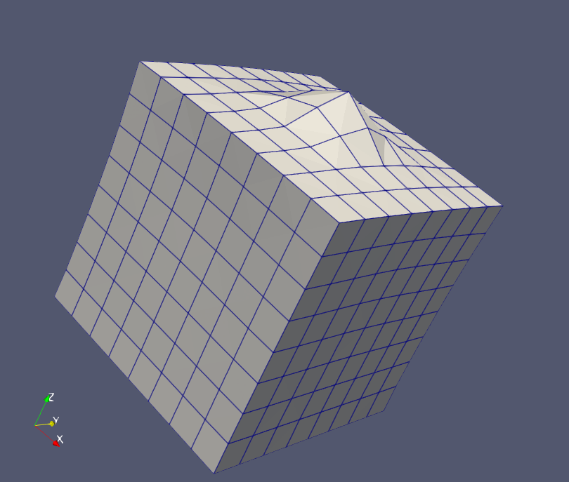
  We got a reaction force -100[N] which is as same as force we added as boundary condition.

  Assemble Body Force

  
  rho_kg_m3 = 7850.0 # the density of steel
  g_m_s2    = 9.81
  gamma_N_m3 = rho_kg_m3 * g_m_s2          # [N/m^3]
  gamma_N_mm3 = gamma_N_m3 / 1e9           # [N/mm^3]
  
  # Constant Body Force along with -Z axis
  f = np.array([0.0, 0.0, -gamma_N_mm3])   # [N/mm^3]
  
  @skfem.LinearForm
  def body(v, w):
      # l(v) = ∫_Ω f · v dΩ
      return dot(f, v)
  
  F_body = body.assemble(basis)