Solve FEM using Gridap with PETSc backend

About

In the previous article, I solved structural analysis with Gridap, which is contained Gridap tutorial, and showed result with vtu file. In this article we extend it to distributed computing with PETSc backend.

Solve Linear Elasticity Problem with Gridap

Code

using Gridap
using GridapPETSc
using GridapDistributed
using PartitionedArrays
using GridapGmsh
path = "./results/script_petsc/"
files_path = path*"data/"
mkpath(files_path)
with_mpi() do distribute
  
  ncpus = 1
  # ncpus = MPI.Comm_size(MPI.COMM_WORLD)
  println("ncpus: ", ncpus)
  ranks = distribute(LinearIndices((ncpus,)))
  # petsc_opts = "-ksp_type cg -pc_type gamg -ksp_rtol 1e-10 -ksp_monitor"
  petsc_opts = "-ksp_type preonly -pc_type lu -ksp_monitor -pc_factor_mat_solver_type superlu_dist"
  GridapPETSc.with(args=split(petsc_opts)) do
    model = GmshDiscreteModel(ranks, "./models/solid.msh")
    order = 1
    reffe = ReferenceFE(lagrangian, VectorValue{3,Float64}, order)
    V0 = TestFESpace(
      model, reffe;
      conformity=:H1,
      dirichlet_tags=["surface_1","surface_2"],
      dirichlet_masks=[(true,false,false), (true,true,true)],
    )
    g1(x) = VectorValue(0.005,0,0) # surface_1: x 方向 5 mm
    g2(x) = VectorValue(0,0,0)     # surface_2: 全拘束
    U = TrialFESpace(V0, [g1,g2])
    # --- 材料定数・応力ひずみ ---
    E = 70.0e9; ν = 0.33
    λ = (E*ν)/((1+ν)*(1-2ν))
    μ =  E/(2*(1+ν))
    # ε(u) = Sym(∇(u))
    σ(ε) = λ*tr(ε)*one(ε) + 2*μ*ε
    # Weak Form
    degree = 2*order
    Ω  = Triangulation(model)
    dΩ = Measure(Ω, degree)
    a(u,v) = ∫( ε(v) ⊙ (σ ∘ ε(u)) )*dΩ
    l(v)   = 0
    op = AffineFEOperator(a, l, U, V0)
    solver = PETScLinearSolver()
    uh = solve(solver, op)
    writevtk(Ω, files_path*"Omega";
      cellfields = [
        "u"     => uh,
        "eps"   => ε(uh),
        "sigma" => σ∘ε(uh)
      ]
    )
  end
end

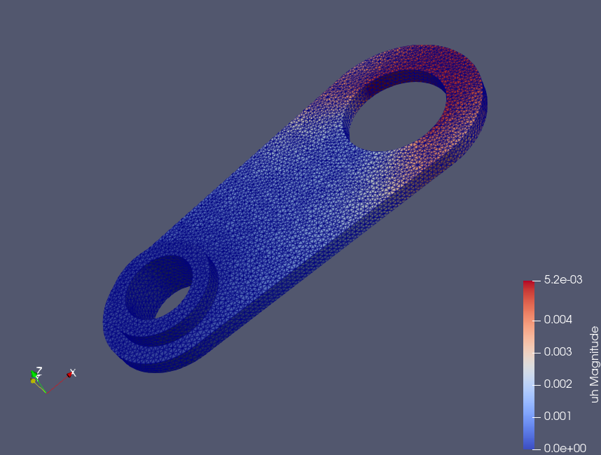
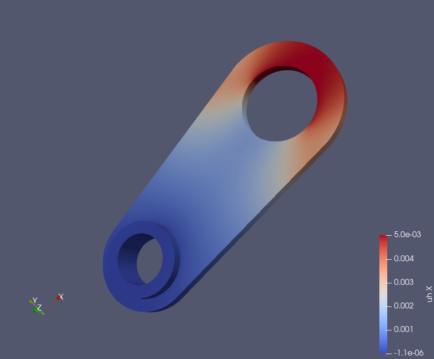
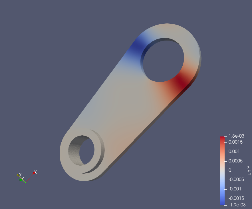
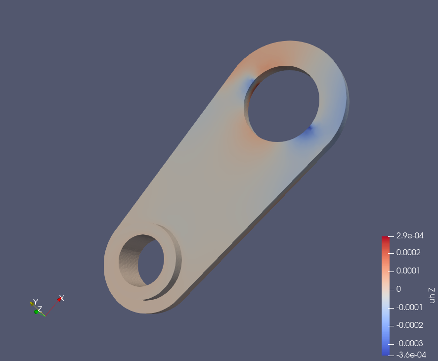
Displacements in each axis

Measure Elapsed Time

start=$(date +%s)
/home/kevin/.julia/bin/mpiexecjl -n 1 \
  julia --project=. script_petsc.jl \
  -on_error_abort -error_output_stderr -ksp_converged_reason
end=$(date +%s)
echo "elapsed time: $((end - start)) sec"
start=$(date +%s)
/home/kevin/.julia/bin/mpiexecjl -n 4 \
  julia --project=. script_petsc.jl \
  -on_error_abort -error_output_stderr -ksp_converged_reason
end=$(date +%s)
echo "elapsed time: $((end - start)) sec"

The scale of this problem

	Single Process	Multi-Process(1)	Multi-Process(4)
# of Cells	40144	as same	as same
# of Points	160576	as same	as same
DoFs (approximate)	481,728	as same	as same

Comparison

	Single Process	Multi-Process(1 – LU)	Multi-Process(4 – LU)	Multi-Process(1 – CG)	Multi-Process(4 – CG)
Elapsed Time[sec]	43	59	61	61	61
Computational Cost	1.0	1.3	1.4	1.4	1.4

But why? Probably, overhead is occurred, and the effect is huge. Or the cost of matrix computation is not dominated.

PETSc Backend

Check PETSc version, config

if you add “-version” as petsc_option, you can see what petsc version behind.

petsc_opts = "-ksp_type cg -pc_type hypre -pc_hypre_type boomeramg -log_view -version"

Petsc Release Version 3.22.0, Sep 28, 2024
       The PETSc Team
    petsc-maint@mcs.anl.gov
 https://petsc.org/
See https://petsc.org/release/changes for recent updates.
See https://petsc.org/release/faq for problems.
See https://petsc.org/release/manualpages for help.
Libraries linked from /workspace/destdir/lib/petsc/double_real_Int64/lib

The version is not the one which I installed custom version of PETSc, I tried to reflect the configuration for GridapPETSc environment.

Install Custom PETSc in your environment

Using below article as reference,

Compile and Install PETSc with external libraries

configure, and do cmake.

./configure \
  --with-openmp=1 \
  --with-debugging=0 \
  --with-shared-libraries=1 \
  --with-mkl_pardiso=1 \
  --with-mkl_pardiso-dir=/opt/intel/oneapi/mkl/2025.2 \
  --with-blaslapack-lib="[/opt/intel/oneapi/mkl/2025.2/lib/libmkl_rt.so,-lpthread,-lm,-ldl]" \
  --download-scalapack \
  --download-superlu_dist \
  --download-mumps \
  --download-hypre \
  --download-mpich \
  --download-cmake \
  COPTFLAGS="-O3 -fopenmp" \
  CXXOPTFLAGS="-O3 -fopenmp" \
  FOPTFLAGS="-O3 -fopenmp"

Put below environment variables, and activated

export PETSC_DIR=$HOME/project/gridap/petsc-3.23.6
export PETSC_ARCH=arch-linux-c-opt
export LD_LIBRARY_PATH=$PETSC_DIR/$PETSC_ARCH/lib:$LD_LIBRARY_PATH
export MKLROOT=/opt/intel/oneapi/mkl/2025.2
export JULIA_PETSC_LIBRARY=$PETSC_DIR/$PETSC_ARCH/lib/libpetsc.so

Re-Build GridapPETSc

export JULIA_PETSC_LIBRARY=$HOME/project/gridap/petsc-3.23.6/arch-linux-c-opt/lib/libpetsc.so
julia --project=. -e 'using Pkg; Pkg.build("GridapPETSc")'

Update the code above with mkl_pardiso backend

using Gridap
using GridapPETSc
using GridapDistributed
using PartitionedArrays
using GridapGmsh

path = "./results/script_petsc/"
files_path = path*"data/"
mkpath(files_path)

petsc_opts = join([
  "-ksp_type preonly",
  "-pc_type lu",
  "-pc_factor_mat_solver_type mkl_pardiso",
  "-ksp_monitor_true_residual",
  "-log_view",
  "-version",
  "-ksp_view_mat ascii:$(files_path)A.mtx:ascii_matrixmarket",
  "-ksp_view_rhs ascii:$(files_path)b.mtx:ascii_matrixmarket",
], " ")

GridapPETSc.with(args=split(petsc_opts)) do

  # model = GmshDiscreteModel(ranks, "./models/solid.msh")
  model = DiscreteModelFromFile("./models/solid.json")

  order = 1
  reffe = ReferenceFE(lagrangian, VectorValue{3,Float64}, order)
  V0 = TestFESpace(
    model, reffe;
    conformity=:H1,
    dirichlet_tags=["surface_1","surface_2"],
    dirichlet_masks=[(true,false,false), (true,true,true)],
  )
  g1(x) = VectorValue(0.005,0,0) # surface_1: x 方向 5 mm
  g2(x) = VectorValue(0,0,0)     # surface_2: 全拘束
  U = TrialFESpace(V0, [g1,g2])

  E = 70.0e9; ν = 0.33
  λ = (E*ν)/((1+ν)*(1-2ν))
  μ =  E/(2*(1+ν))
  # ε(u) = Sym(∇(u))
  σ(ε) = λ*tr(ε)*one(ε) + 2*μ*ε

  # Weak Form
  degree = 2*order
  Ω  = Triangulation(model)
  dΩ = Measure(Ω, degree)

  a(u,v) = ∫( ε(v) ⊙ (σ ∘ ε(u)) )*dΩ
  l(v)   = 0
  op = AffineFEOperator(a, l, U, V0)

  solver = PETScLinearSolver()
  uh = solve(solver, op)

  writevtk(Ω, files_path*"Omega";
    cellfields = [
      "u"     => uh,
      "eps"   => ε(uh),
      "sigma" => σ∘ε(uh)
    ]
  )
end

Run GridapPETSc under options

petsc_opts = "-ksp_type preonly -pc_type lu -pc_factor_mat_solver_type mkl_pardiso -ksp_monitor_true_residual -log_view -version"
# When you would like to use iterative method CG
# petsc_opts = "-ksp_type cg -pc_type hypre -pc_hypre_type boomeramg -log_view -version"

and run julia with script.jl.

MKL_NUM_THREADS=8 OMP_NUM_THREADS=8 OPENBLAS_NUM_THREADS=8 julia --project=. script.jl 

It does not get much faster, but multi-threading was activated, and multiple cpus are used. The bottleneck of this code is not in the matrix computation. According to PETSc stats when we use direct method, which is LU, computation with 8 threads is much faster. But as you can see, total time is much higher than computation time. It is probably because it uses much resources for assembling matrix etc.

	1 Thread	8 Threads
MatLUFactorNum[sec]	0.229	0.0437
PCSetUp[sec]	0.411	0.19
KSPSolve[sec]	0.011	0.0070
Total[sec]	31.1	31.0

When we see stats when we use CG method with hypre backend,

	1 Thread	8 Thread
KSPSolve[sec]	15.7	8.4
PCApply(HYPRE BoomerAMG PreProcessing)[sec]	15.6	8.2
MatMult[sec]	0.148	0.161
Total[sec]	47.22	39.47

Even it gets slower. I should test the setting under more large problem.