Introduction
GridapTopOpt is a library that is able to handle level set method based topology optimization. This library is built with Gridap family, which enables us to do with finite element analysis, can be run as multiple processing ( or threading) with MPI. The code is implemented with a little bit old version of Gridap, and I would like to run it with PETSc multi-threading, I revised their tutorial code.
Code
In their code,
using Gridap, Gridap.Geometry, Gridap.Adaptivity, Gridap.MultiField, Gridap.TensorValues
using GridapEmbedded, GridapEmbedded.LevelSetCutters
using GridapSolvers, GridapSolvers.BlockSolvers, GridapSolvers.NonlinearSolvers
using GridapGmsh
using PartitionedArrays
using GridapPETSc
using GridapTopOpt
using Gridap.FESpaces: get_fe_space, get_cell_dof_ids
using Gridap.FESpaces: FEFunction
using GridapTopOpt: StateParamMap
"""
This example appears in our manuscript:
"Level-set topology optimisation with unfitted finite elements and automatic shape differentiation"
by Z.J. Wegert, J. Manyer, C. Mallon, S. Badia, V.J. Challis. (10.1016/j.cma.2025.118203)
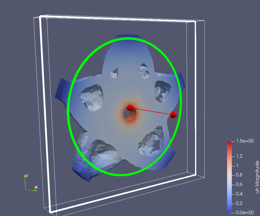
(MPI) Three-dimensional minimum elastic compliance of a wheel using a CutFEM formulation based
on Burman et al. (2018) [10.1016/j.cma.2017.09.005] & automatic shape differentiation.
Optimisation problem:
Min J(Ω) = ∫ ε(d) ⊙ σ(ε(d)) dΩ
Ω
s.t., Vol(Ω) = 0.3,
⎡d∈V=H¹(Ω;u(Γ_D)=0),
⎣∫ ε(s) ⊙ σ ∘ ε(d) dΩ + j(d,s) + i(d,s) = ∫ s⋅g dΓ_N, ∀v∈V.
In the above, j(d,s) is the ghost penalty term over the ghost skeleton Γg
with outward normal n_Γg, and i(d,s) enforces zero temperature within the
isolated volumes marked by χ. These are given by
j(d,s) = ∫ γh³[[∇(d)⋅n_Γg]]⋅[[(∇(s)⋅n_Γg]] dΓg, &
i(d,s) = ∫ χd ⋅ s dΩ.
"""
function main()
# Params
vf = 0.5
γ_evo = 0.1
max_steps = 10
# vf = 0.3
# α_coeff = 1.0
α_coeff = γ_evo*max_steps
iter_mod = 50
D = 3
mesh_name = "Wheel_3d_a.msh"
mesh_file = (@__DIR__)*"/Meshes/$mesh_name"
# Output path
path = "./results/Wheel3D_CutFEM_org_b/"
files_path = path*"data/"
model_path = path*"model/"
mkpath(files_path); mkpath(model_path);
# Load mesh
model = GmshDiscreteModel(mesh_file)
model = UnstructuredDiscreteModel(model)
f_diri(x) =
((cos(30π/180)<=x[1]<=cos(15π/180)) && abs(x[2] - sqrt(1-x[1]^2))<1e-4) ||
((cos(97.5π/180)<=x[1]<=cos(82.5π/180)) && abs(x[2] - sqrt(1-x[1]^2))<1e-4) ||
((cos(165π/180)<=x[1]<=cos(150π/180)) && abs(x[2] - sqrt(1-x[1]^2))<1e-4) ||
((cos(142.5π/180)<=x[1]<=cos(127.5π/180)) && abs(x[2] - -sqrt(1-x[1]^2))<1e-4) ||
((cos(52.5π/180)<=x[1]<=cos(37.5π/180)) && abs(x[2] - -sqrt(1-x[1]^2))<1e-4)
update_labels!(1,model,f_diri,"Gamma_D_new")
writevtk(model,model_path*"model")
# Get triangulation and element size
Ω_bg = Triangulation(model)
hₕ = get_element_diameter_field(model)
hmin = minimum(get_element_diameters(model))
# Cut the background model
reffe_scalar = ReferenceFE(lagrangian,Float64,1)
V_φ = TestFESpace(model,reffe_scalar)
V_reg = TestFESpace(model,reffe_scalar;dirichlet_tags=["Gamma_N",])
U_reg = TrialFESpace(V_reg)
_f1((x,y,z),q,r) = - cos(q*π*x)*cos(q*π*y)*cos(q*π*z)/q - r/q
_f2((x,y,z)) = -sqrt(x^2+y^2)+0.9
φh = interpolate(x->min(_f1(x,4,0.1),_f2(x)),V_φ)
# Check LS
GridapTopOpt.correct_ls!(φh)
# Setup integration meshes and measures
order = 1
degree = 2*(order+1)
Γ_N = BoundaryTriangulation(model,tags=["Gamma_N",])
dΓ_N = Measure(Γ_N,degree)
dΩ_bg = Measure(Ω_bg,degree)
Ω_data = EmbeddedCollection(model,φh) do cutgeo,cutgeo_facets,_φh
Ω = DifferentiableTriangulation(Triangulation(cutgeo,PHYSICAL),V_φ)
Γ = DifferentiableTriangulation(EmbeddedBoundary(cutgeo),V_φ)
Γg = GhostSkeleton(cutgeo)
Ω_act = Triangulation(cutgeo,ACTIVE)
# Isolated volumes
# φ_cell_values = map(get_cell_dof_values,local_views(_φh))
# FEFunction φh の所属する FESpace を取得
space = get_fe_space(_φh)
# セルごとの DOF インデックスを取得
cell_ids = get_cell_dof_ids(space)
# φh の DOF 値のベクトルを取得
u_vec = get_free_dof_values(_φh)
# 各セルごとの DOF 値を抽出
φ_cell_values = [u_vec[ids] for ids in cell_ids]
ψ,_ = get_isolated_volumes_mask_polytopal(model,φ_cell_values,["Gamma_D_new",])
(;
:Ω_act => Ω_act,
:Ω => Ω,
:dΩ => Measure(Ω,degree),
:Γg => Γg,
:dΓg => Measure(Γg,degree),
:n_Γg => get_normal_vector(Γg),
:Γ => Γ,
:dΓ => Measure(Γ,degree),
:n_Γ => get_normal_vector(Γ),
:ψ => ψ
)
end
# Setup spaces
reffe_d = ReferenceFE(lagrangian,VectorValue{D,Float64},order)
function build_spaces(Ω_act)
V = TestFESpace(Ω_act,reffe_d,conformity=:H1,dirichlet_tags=["Gamma_D_new",])
U = TrialFESpace(V)
return U,V
end
### Weak form
# Material parameters
function lame_parameters(E,ν)
λ = (E*ν)/((1+ν)*(1-2*ν))
μ = E/(2*(1+ν))
(λ, μ)
end
λs, μs = lame_parameters(1.0,0.3)
α_Gd = 1e-7
k_d = 1.0
# α_Gd = 3e-5
# k_d = 10.0
γ_Gd(h) = α_Gd*(λs + μs)*h^3
# Terms
σ(ε) = λs*tr(ε)*one(ε) + 2*μs*ε
a_s_Ω(d,s) = ε(s) ⊙ (σ ∘ ε(d)) # Elasticity
j_s_k(d,s) = mean(γ_Gd ∘ hₕ)*(jump(Ω_data.n_Γg ⋅ ∇(s)) ⋅ jump(Ω_data.n_Γg ⋅ ∇(d)))
v_s_ψ(d,s) = (k_d*Ω_data.ψ)*(d⋅s) # Isolated volume term
g((x,y,z)) = 100VectorValue(-y,x,0.0)
a(d,s,φ) = ∫(a_s_Ω(d,s) + v_s_ψ(d,s))Ω_data.dΩ + ∫(j_s_k(d,s))Ω_data.dΓg
l(s,φ) = ∫(s⋅g)dΓ_N
## Optimisation functionals
vol_D = sum(∫(1)dΩ_bg)
J_comp(d,φ) = ∫(ε(d) ⊙ (σ ∘ ε(d)))Ω_data.dΩ
Vol(d,φ) = ∫(1/vol_D)Ω_data.dΩ - ∫(vf/vol_D)dΩ_bg
dVol(q,d,φ) = ∫(-1/vol_D*q/(abs(Ω_data.n_Γ ⋅ ∇(φ))))Ω_data.dΓ
## Setup solver and FE operators
elast_ls = PETScLinearSolver(lu_pardiso_ksp_setup())
state_collection = EmbeddedCollection_in_φh(model,φh) do _φh
update_collection!(Ω_data,_φh)
U,V = build_spaces(Ω_data.Ω_act)
state_map = AffineFEStateMap(a,l,U,V,V_φ;ls=elast_ls,adjoint_ls=elast_ls)
(;
:state_map => state_map,
:J => StateParamMap(J_comp,state_map),
:C => map(Ci -> StateParamMap(Ci,state_map),[Vol,])
)
end
pcf = EmbeddedPDEConstrainedFunctionals(state_collection;analytic_dC=(dVol,))
## Evolution Method
# evolve_ls = PETScLinearSolver()
evolve_ls = PETScLinearSolver(lu_pardiso_ksp_setup())
evolve_nls = NewtonSolver(evolve_ls;maxiter=1,verbose=true)
# evolve_nls = NewtonSolver(evolve_ls;maxiter=5,verbose=true)
# reinit_nls = NewtonSolver(PETScLinearSolver();maxiter=20,rtol=1.e-14,verbose=true)
reinit_nls = NewtonSolver(PETScLinearSolver(lu_pardiso_ksp_setup());maxiter=20,rtol=1.e-14,verbose=true)
evo = CutFEMEvolver(V_φ,Ω_data,dΩ_bg,hₕ;max_steps,γg=0.01,ode_ls=evolve_ls,ode_nl=evolve_nls)
reinit = StabilisedReinitialiser(V_φ,Ω_data,dΩ_bg,hₕ;stabilisation_method=ArtificialViscosity(0.5),nls=reinit_nls)
# reinit = StabilisedReinitialiser(V_φ,Ω_data,dΩ_bg,hₕ;stabilisation_method=ArtificialViscosity(0.1),nls=reinit_nls)
ls_evo = LevelSetEvolution(evo,reinit)
## Hilbertian extension-regularisation problems
hilb_ls = CGAMGSolver()
α_floor = 1e-6
_α(hₕ) = (α_coeff*hₕ)^2 + α_floor
# _α(hₕ) = (α_coeff*hₕ)^2
a_hilb(p,q) =∫((_α ∘ hₕ)*∇(p)⋅∇(q) + p*q)dΩ_bg;
vel_ext = VelocityExtension(a_hilb,U_reg,V_reg;ls=hilb_ls)
## Optimiser
converged(m) = GridapTopOpt.default_al_converged(
m;
L_tol = 0.01hmin,
C_tol = 0.01
)
optimiser = AugmentedLagrangian(pcf,ls_evo,vel_ext,φh;
γ=γ_evo,verbose=true,constraint_names=[:Vol],converged)
println("optimiser")
for (it,uh,φh) in optimiser
# @info "it/iter_mod = $(it) / $(iter_mod)"
@info "iter = $(it)"
# if iszero(it % iter_mod)
writevtk(Ω_bg,files_path*"Omega_act_$it",
cellfields=["φ"=>φh,"|∇(φ)|"=>(norm ∘ ∇(φh)),"uh"=>uh,"ψ"=>Ω_data.ψ])
writevtk(Ω_data.Ω,files_path*"Omega_in_$it",cellfields=["uh"=>uh])
# end
psave(files_path*"LSF_$it",get_free_dof_values(φh))
write_history(path*"/history.txt",optimiser.history;ranks)
end
println("it = get_history")
it = get_history(optimiser).niter; uh = get_state(pcf)
writevtk(Ω_bg,path*"Omega_act_$it",cellfields=["φ"=>φh,"|∇(φ)|"=>(norm ∘ ∇(φh)),"uh"=>uh,"ψ"=>Ω_data.ψ])
writevtk(Ω_data.Ω,path*"Omega_in_$it",cellfields=["uh"=>uh])
psave(path*"LSF_$it",get_free_dof_values(φh))
nothing
end
## CG-AMG solver
CGAMGSolver(;kwargs...) = PETScLinearSolver(gamg_ksp_setup(;kwargs...))
function gamg_ksp_setup(;rtol=10^-8,maxits=100)
function ksp_setup(ksp)
pc = Ref{GridapPETSc.PETSC.PC}()
rtol = PetscScalar(rtol)
atol = GridapPETSc.PETSC.PETSC_DEFAULT
dtol = GridapPETSc.PETSC.PETSC_DEFAULT
maxits = PetscInt(maxits)
@check_error_code GridapPETSc.PETSC.KSPSetType(ksp[],GridapPETSc.PETSC.KSPCG)
@check_error_code GridapPETSc.PETSC.KSPSetTolerances(ksp[], rtol, atol, dtol, maxits)
@check_error_code GridapPETSc.PETSC.KSPGetPC(ksp[],pc)
@check_error_code GridapPETSc.PETSC.PCSetType(pc[],GridapPETSc.PETSC.PCGAMG)
@check_error_code GridapPETSc.PETSC.KSPView(ksp[],C_NULL)
end
return ksp_setup
end
function lu_pardiso_ksp_setup(; rtol=1e-8, maxits=100)
function ksp_setup(ksp)
pc = Ref{GridapPETSc.PETSC.PC}()
# 収束条件
rtol = PetscScalar(rtol)
atol = GridapPETSc.PETSC.PETSC_DEFAULT
dtol = GridapPETSc.PETSC.PETSC_DEFAULT
maxits = PetscInt(maxits)
# KSP を preonly に
@check_error_code GridapPETSc.PETSC.KSPSetType(ksp[], GridapPETSc.PETSC.KSPPREONLY)
@check_error_code GridapPETSc.PETSC.KSPSetTolerances(ksp[], rtol, atol, dtol, maxits)
# PC を LU に
@check_error_code GridapPETSc.PETSC.KSPGetPC(ksp[], pc)
@check_error_code GridapPETSc.PETSC.PCSetType(pc[], GridapPETSc.PETSC.PCLU)
# factorization solver type を MKL Pardiso に
# (エラーが出る場合はここを MUMPS/SuperLU_DIST に変える)
@check_error_code GridapPETSc.PETSC.PCFactorSetMatSolverType(pc[], "mkl_pardiso")
# デバッグ用に KSPView
@check_error_code GridapPETSc.PETSC.KSPView(ksp[], C_NULL)
end
return ksp_setup
end
## Run
GridapPETSc.with() do
main()
end
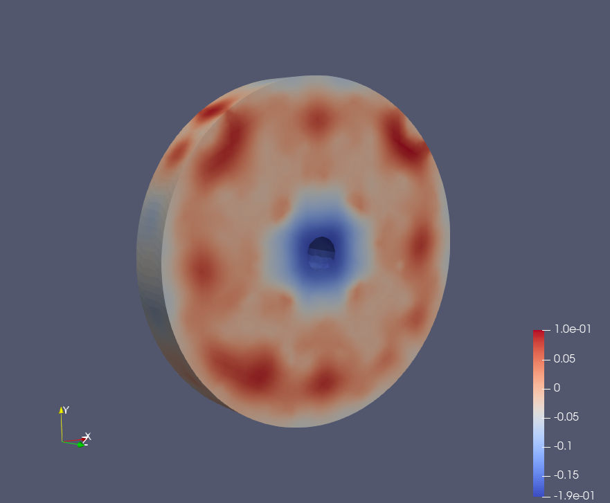
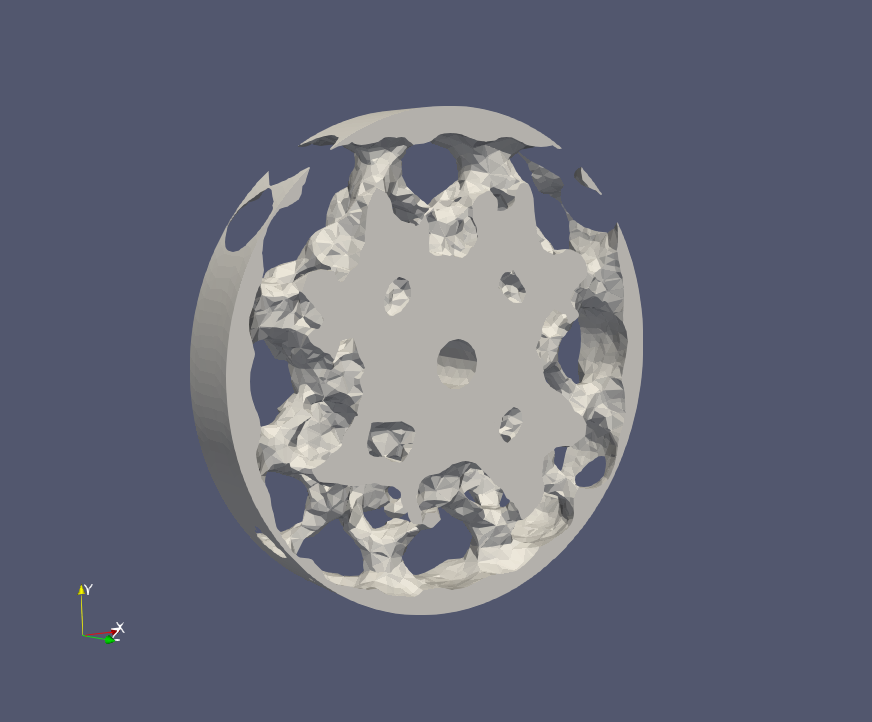
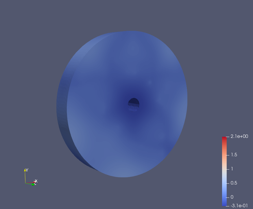
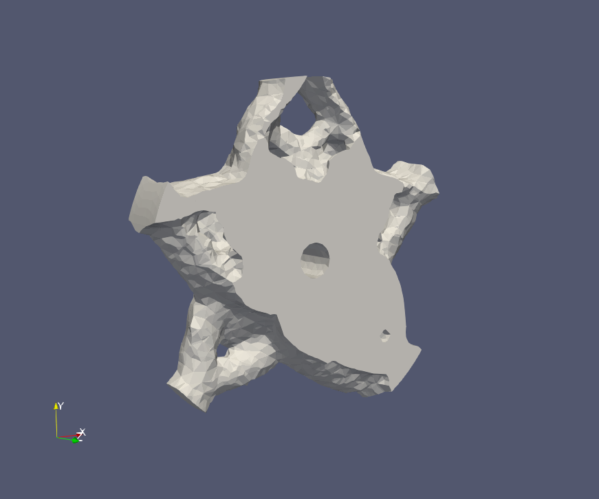
Result
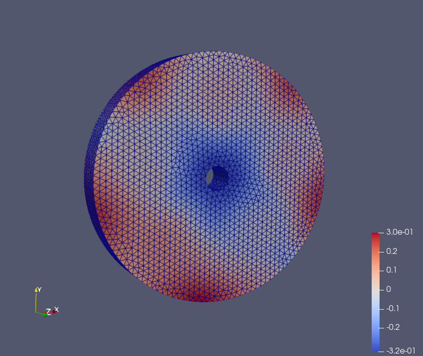
The number of cells and Points are 36552 and 146208.
Epoch: 1
Epoch: 15
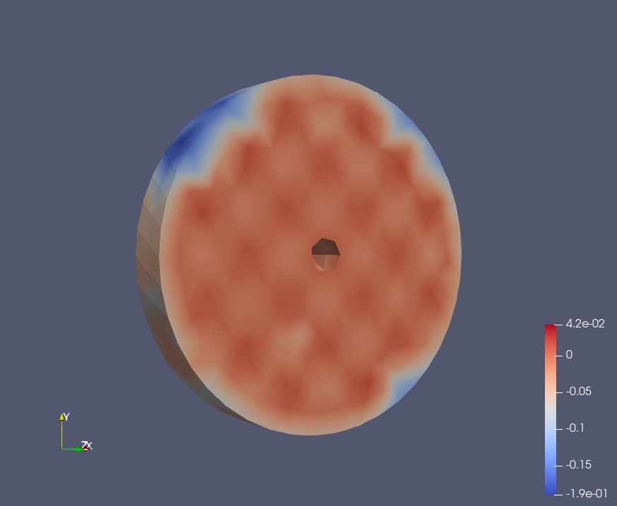
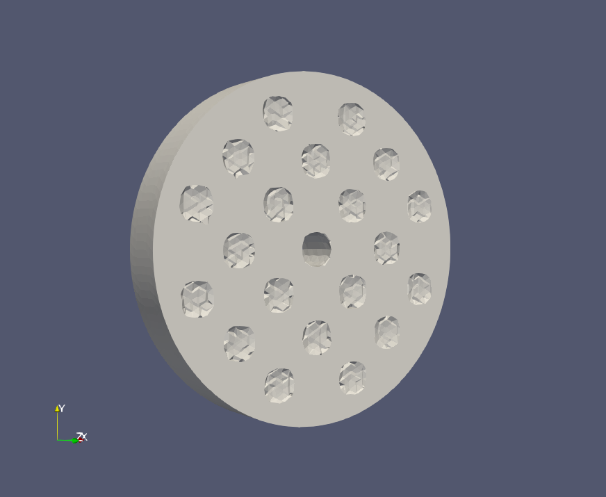
Epoch: 40
Epoch: 60
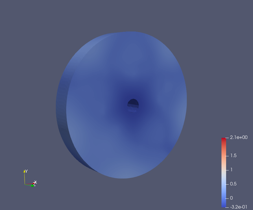
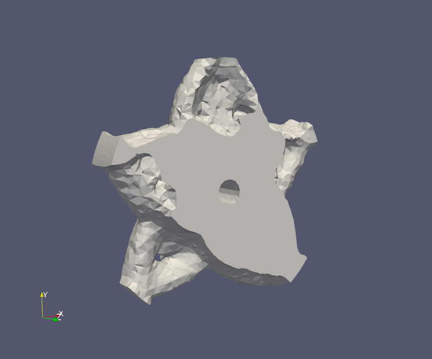
Intersection and Displacement