Solve Linear Elasticity with Gridap, Julia

About

Gridap is a highly useful finite element solver built with Julia.
However, since the documentation still feels somewhat incomplete, I decided to implement and summarize some code that could serve as commonly used templates. The task I worked on was solving linear structural analysis problems.

Even though structural analysis may sound straightforward, executing it correctly requires effort. You need to write the code and then verify numerically that the results are valid.

Implementation

The simulation itself is very simple: one end of a flat plate is fixed, and the opposite end is pulled.

using Gridap, Gridap.TensorValues, LinearAlgebra
using Gridap.Geometry
using Logging

function set_logger_from_args(args)
    level = get(ARGS, 1, "info")
    lvl = Dict(
        "debug" => Logging.Debug,
        "info"  => Logging.Info,
        "warn"  => Logging.Warn,
        "error" => Logging.Error
    )[lowercase(level)]
    global_logger(ConsoleLogger(stderr, lvl))
end

set_logger_from_args(ARGS)

files_path = "results/linear_elasticity/"
mkpath(files_path)
order  = 1
degree = 2*order


Lx, Ly, Lz = (5.0, 5.0, 1.0)
nx, ny, nz = (10, 10, 2)
domain = (0.0,Lx, 0.0,Ly, 0.0,Lz)
partition = (nx,ny,nz)
model = CartesianDiscreteModel(domain, partition)

d = num_cell_dims(model)
Ω  = Triangulation(model)
Γ  = BoundaryTriangulation(Ω)
labels = get_face_labeling(model)
tol = 1e-5
tol_rough = 0.3

topo   = get_grid_topology(model)
toplab = Gridap.Geometry.face_labeling_from_vertex_filter(
  topo, "surface_top", x -> isapprox(x[2], Ly; atol=tol)
)
bottomlab = Gridap.Geometry.face_labeling_from_vertex_filter(
  topo, "surface_bottom", x -> isapprox(x[2], 0.0; atol=tol)
)

merge!(labels, toplab)
merge!(labels, bottomlab)

∂Ω = Measure(Ω, degree)
∂Γ = Measure(Γ, degree)

println("Registered Tags: ", labels.tag_to_name)


reffe = ReferenceFE(lagrangian, VectorValue{3,Float64}, order)
Vfree = TestFESpace(model, reffe; conformity=:H1)
V = TestFESpace(
    model, reffe; conformity=:H1,
    dirichlet_tags=["surface_bottom"],
    dirichlet_masks=[(true,true,true)]
)

@show num_free_dofs(Vfree), num_free_dofs(V)

g(x) = VectorValue(0.0,0.0,0.0)
U = TrialFESpace(V, [g])

E  = 210e9
ν  = 0.3
λ  = (E*ν)/((1+ν)*(1-2ν))
μ  = E/(2*(1+ν))
ε(u) = symmetric_gradient(u)
# ε(u) = 0.5*(∇(u) + ∇(u)')
dim = num_cell_dims(model)  # 2 or 3

# ε(u) = symmetric(∇(u))
I    = one(TensorValue{dim,dim,Float64})
σ(u) = λ*tr(ε(u))*I + 2μ*ε(u)


pa = 1e6
Γtop  = BoundaryTriangulation(
    Ω;
    tags=["surface_top"]
)
∂Γtop = Measure(Γtop, degree)
@info "num Γtop cells" num_cells(Γtop)
A_top = sum( ∫( 1.0 )∂Γtop )[1]
@info "Γtop area" A_top

n_top = Gridap.CellData.get_normal_vector(Γtop)
l(v) = ∫( pa * (v ⋅ n_top) )∂Γtop
a(u,v) = ∫( ε(v) ⊙ σ(u) )∂Ω

op = AffineFEOperator(a, l, U, V)

uh = solve(op)

εh = ε(uh)
σh = σ(uh)
wh = 0.5*(εh ⊙ σh)

writevtk(
  Ω, files_path*"elasticity_all";
  cellfields = [
    "u" => uh,
    "epsilon" => εh,              # εh = ε(uh)
    "sigma" => σh,                # σh = σ(uh)
    "strain_energy" => wh         # wh = 0.5*(εh ⊙ σh)
  ],
)

d = num_cell_dims(model) - 1
mask_top_global    = get_face_mask(labels, "surface_top",    d)
mask_bottom_global = get_face_mask(labels, "surface_bottom", d)
mask_boundary_global = get_isboundary_face(topo, d) 
boundary_dface_ids = findall(mask_boundary_global)

# global -> local
mask_top_local    = mask_top_global[boundary_dface_ids]
mask_bottom_local = mask_bottom_global[boundary_dface_ids]

writevtk(
  Γ, files_path*"boundary_tags";
  cellfields = [
    "surface_top"    => CellField(Float32.(mask_top_local), Γ),
    "surface_bottom" => CellField(Float32.(mask_bottom_local), Γ),
  ],
)

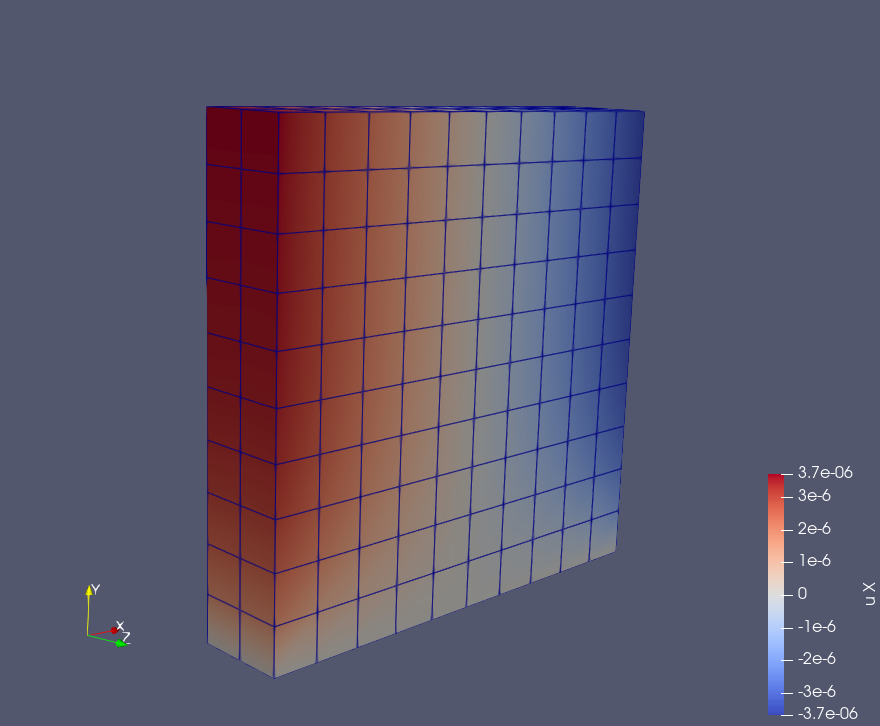
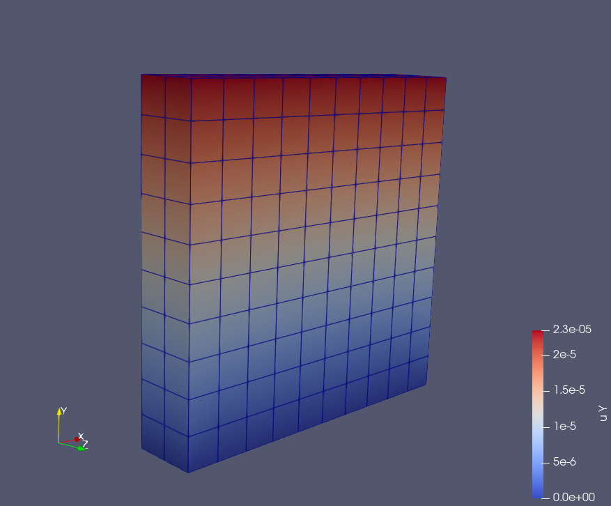
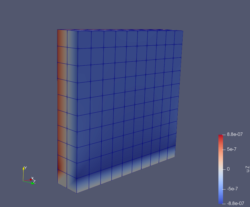
Result

Displacement in XYZ axis

Thought

In practice, I felt that Gridap is user-friendly, provided one has an understanding of the structure of the finite element method.
However, the distinction between global and local indices is extremely difficult to grasp. In addition, there seems to be little information on where exactly data are stored and which functions should be used to retrieve them. As mentioned earlier, verifying reliability is important.