
Introduction
Since Julia has great package Gridap, which is able to deal with FEM computation efficiently, Julia lang is one of the candidates for engineers or researchers to do physics simulation. But we should know what kind of means is the best option to solve the linear equations that are provided by FEM. For sure, there are great library, which are GridapPETSc or Distributed.jl, enables us to solver equations with distributed computing. But the options are sometimes inefficient for some cases. for example, when the number of DoFs is less than million, or we do not have so many computers that can be accessed. Therefore, what this article is going to clarify is how libraries in Julia lang are able to speed up the computation with multi-threading.
In the below article, I tried solving multiple linear equations with Scipy and Joblib. By using Joblib, we can solve multiple equations simultaneously with multi-threading. This is absolutely great and worth to use in many cases, but it is NOT able to solve single linear equation with multi-threading as Scipy is not able to handle multi-threading basically.
One of the advantage of using Julia to solve linear equation is that it is able to solve single linear equation with multi-threading.
To be precise, the explanation above is slightly different from how things actually work.
Both SciPy (Python) and LinearAlgebra (Julia) rely on BLAS as their backend.
However, while it is difficult to explicitly control the degree of parallelism from SciPy, Julia makes it much easier to manage directly from code.
What I test in this experiment
The content of experiment
The program benchmarks the performance of different solvers for linear systems on both dense and sparse matrices. It solves the systems using LU decomposition, Cholesky factorization, QR decomposition, and iterative methods, measures the computation time, and outputs comparison plots.
Scenarios
Dense SPD case: A symmetric positive definite dense matrix is solved using LU, Cholesky, QR, and the Conjugate Gradient method.
Dense General case: A general dense matrix is solved using LU, QR, and the GMRES iterative method.
Sparse SPD case: A sparse symmetric positive definite matrix is solved using UMFPACK (sparse LU), CHOLMOD (sparse Cholesky), SPQR (sparse QR), and Conjugate Gradient.
Sparse General case: A general sparse matrix is solved using UMFPACK, SPQR, and GMRES.
Code
# =========================
# benchmark_solvers.jl
# =========================
using LinearAlgebra
using SparseArrays
using SuiteSparse
using BenchmarkTools
using IterativeSolvers
using Random
using Plots

module _KrylovCompat
using IterativeSolvers

"cg を常にベクトル返しで統一(reltol系/rol系どちらも対応)"
function cg_vec(A, b; tol=1e-8, maxiter=10_000)
    # 新しめAPI(reltol)
    try
        x = IterativeSolvers.cg(A, b; reltol=tol, maxiter=maxiter, log=false)
        return x
    catch
        # 旧API(tol)
        x = IterativeSolvers.cg(A, b; tol=tol, maxiter=maxiter, log=false)
        return x
    end
end

"gmres を常にベクトル返しで統一(返り値が x か (x,stats) かの差異を吸収)"
function gmres_vec(A, b; tol=1e-8, maxiter=10_000)
    # 新しめAPI(reltol)
    try
        res = IterativeSolvers.gmres(A, b; reltol=tol, maxiter=maxiter, log=false)
        return res isa Tuple ? res[1] : res
    catch
        # 旧API(tol)
        res = IterativeSolvers.gmres(A, b; tol=tol, maxiter=maxiter, log=false)
        return res isa Tuple ? res[1] : res
    end
end

end
const KC = _KrylovCompat


# ---- 環境設定(必要に応じて) ----
# BLASスレッドは疎行列計算では効果が薄いので 1 を推奨
BLAS.set_num_threads(1)
# CHOLMOD / SPQR の OpenMP スレッド数(必要に応じて)
try
    SuiteSparse.CHOLMOD.set_nthreads(Sys.CPU_THREADS)
    SuiteSparse.SPQR.set_nthreads(Sys.CPU_THREADS)
catch
end

# ==== ユーティリティ ====
# SPD な密行列
function make_dense_SPD(n; seed=0)
    seed != nothing && Random.seed!(seed)
    A = randn(n, n)
    A = A' * A               # 対称正定値
    A += n * I               # 条件を少し良く
    Symmetric(A)
end

# 一般(非対称でもよい)密行列
function make_dense_general(n; seed=0)
    seed != nothing && Random.seed!(seed)
    randn(n, n)
end

# SPD な疎行列
# function make_sparse_SPD(n; density=5/n, seed=0)
#     seed != nothing && Random.seed!(seed)
#     S = sprand(n, n, density)
#     A = S + S' + spdiagm(0 => fill(10.0, n))  # 対称かつ対角優位で実質SPD
#     Symmetric(A)
# end
function make_sparse_SPD(n; density=0.01, seed=nothing)
    if seed !== nothing
        Random.seed!(seed)
    end
    A = sprand(n, n, density)
    A = A + transpose(A)
    A = A + n * I
    return A
end

function make_sparse_general(n; density=5/n, seed=0)
    seed !== nothing && Random.seed!(seed)
    A = sprand(n, n, density)
    # A += spdiagm(0 => fill(1e-3, n))
    A = A + n * I
    return A
end
function generate_random_spd_matrix(n; density=0.01, seed=nothing)
    if seed !== nothing
        Random.seed!(seed)
    end
    A = sprand(n, n, density)
    A = A + transpose(A)
    A = A + n * I
    return A
end


# 複数右辺
make_rhs(n, nrhs; seed=0) = (seed != nothing && Random.seed!(seed); randn(n, nrhs))

# ==== 測定ヘルパ ====
# 単一関数をベンチ → 経過秒を返す
function timeit(f; samples=3, evals=1)
    res = @benchmark $f() samples=samples evals=evals
    return minimum(res).time * 1e-9  # ns → 秒
end

# ==== 密行列:SPD ケース(LU vs Cholesky vs QR vs CG)====
function bench_dense_SPD(n, nrhs; samples=3, seed=0, cg_tol=1e-8, cg_maxiter=10_000)
    A = make_dense_SPD(n; seed)
    B = make_rhs(n, nrhs; seed=seed+1)

    # 事前ウォームアップ
    _ = A \ B

    results = Dict{String,Float64}()

    # LU(通常解法)
    results["Dense LU"] = timeit(() -> (F=lu(A); X = F \ B); samples=samples)

    # Cholesky(方法1)
    results["Dense Cholesky"] = timeit(() -> (F=cholesky(A; check=false); X = F \ B); samples=samples)

    # QR(方法2)
    results["Dense QR"] = timeit(() -> (F=qr(Matrix(A)); X = F \ B); samples=samples)

    # 反復法 CG(方法3)— SPD 用
    results["Dense CG"] = timeit(() -> begin
        X = similar(B)
        for j in axes(B, 2)
            X[:, j] = cg(A, B[:, j]; reltol=cg_tol, maxiter=cg_maxiter, log=false)
        end
    end; samples=samples)

    results
end

# ==== 密行列:一般ケース(LU vs QR vs GMRES)====
function bench_dense_general(n, nrhs; samples=3, seed=0, gmres_tol=1e-8, gmres_maxiter=10_000)
    A = make_dense_general(n; seed)
    B = make_rhs(n, nrhs; seed=seed+1)

    results = Dict{String,Float64}()

    results["Dense LU"] = timeit(() -> (F=lu(A); X = F \ B); samples=samples)
    results["Dense QR"] = timeit(() -> (F=qr(A); X = F \ B); samples=samples)

    results["Dense GMRES"] = timeit(() -> begin
        X = similar(B)
        for j in axes(B, 2)
            x = KC.gmres_vec(A, B[:, j]; tol=gmres_tol, maxiter=gmres_maxiter)
            @assert x isa AbstractVector
            copy!(view(X, :, j), x)
        end
    end; samples=samples)


    results
end

# ==== 疎行列:SPD ケース(UMFPACK-LU vs CHOLMOD vs SPQR vs CG)====
function bench_sparse_SPD(n, nrhs; density=5/n, samples=3, seed=0, cg_tol=1e-8, cg_maxiter=100_000)
    A = make_sparse_SPD(n; density, seed)
    B = make_rhs(n, nrhs; seed=seed+1)

    results = Dict{String,Float64}()

    # UMFPACK の LU(通常)
    results["Sparse LU (UMFPACK)"] = timeit(() -> (F=lu(A); X = F \ B); samples=samples)

    # CHOLMOD(方法1)
    results["Sparse Cholesky (CHOLMOD)"] = timeit(() -> (F=cholesky(A; check=false); X = F \ B); samples=samples)

    # SPQR(方法2)— SPD でも動くが過剰、比較用
    results["Sparse QR (SPQR)"] = timeit(() -> (F=qr(A); X = F \ B); samples=samples)

    # CG(方法3)
    results["Sparse CG"] = timeit(() -> begin
        X = similar(B)
        for j in axes(B, 2)
            X[:, j] = cg(A, B[:, j]; reltol=cg_tol, maxiter=cg_maxiter, log=false)
        end
    end; samples=samples)

    results
end

# ==== 疎行列:一般ケース(UMFPACK-LU vs SPQR vs GMRES)====
function bench_sparse_general(n, nrhs; density=5/n, samples=3, seed=0, gmres_tol=1e-8, gmres_maxiter=100_000)
    A = make_sparse_general(n; density, seed)
    B = make_rhs(n, nrhs; seed=seed+1)

    results = Dict{String,Float64}()

    results["Sparse LU (UMFPACK)"] = timeit(() -> (F=lu(A); X = F \ B); samples=samples)
    results["Sparse QR (SPQR)"] = timeit(() -> (F=qr(A); X = F \ B); samples=samples)

    results["Sparse GMRES"] = timeit(() -> begin
        X = similar(B)
        for j in axes(B, 2)
            x = KC.gmres_vec(A, B[:, j]; tol=gmres_tol, maxiter=gmres_maxiter)
            @assert x isa AbstractVector
            copy!(view(X, :, j), x)
        end
    end; samples=samples)


    results
end

# ==== プロットユーティリティ ====
function plot_results(dicts::Vector{Dict{String,Float64}}, titles::Vector{String})
    @assert length(dicts) == length(titles)
    plots = Vector{Plots.Plot{Plots.GRBackend}}(undef, length(dicts))
    for (i, (d, ttl)) in enumerate(zip(dicts, titles))
        labels = collect(keys(d))
        times  = [d[k] for k in labels]
        # 並びを見やすく(速い順)
        pidx = sortperm(times)
        labels = labels[pidx]
        times  = times[pidx]
        plots[i] = bar(labels, times; legend=false, xlabel="Method", ylabel="Time [s]", title=ttl, xrotation=20)
    end
    return plot(plots...; layout=(2,2), size=(1000,800))
end

# ==== メイン:サイズや密度を変えて実行 ====
function main(; n_dense=2000, n_sparse=50_000, nrhs=4, density=10/n_sparse, samples=3, seed=0)
    println("== Dense SPD ==")
    d1 = bench_dense_SPD(n_dense, nrhs; samples=samples, seed=seed)
    println(d1)
    println("== Dense General ==")
    d2 = bench_dense_general(n_dense, nrhs; samples=samples, seed=seed+10)
    println(d2)
    println("== Sparse SPD ==")
    s1 = bench_sparse_SPD(n_sparse, nrhs; density=density, samples=samples, seed=seed+20)
    println(s1)
    println("== Sparse General ==")
    s2 = bench_sparse_general(n_sparse, nrhs; density=density, samples=samples, seed=seed+30)
    println(s2)

    plt = plot_results([d1, d2, s1, s2],
        ["Dense SPD (LU vs Cholesky vs QR vs CG)",
        "Dense General (LU vs QR vs GMRES)",
        "Sparse SPD (UMFPACK vs CHOLMOD vs SPQR vs CG)",
        "Sparse General (UMFPACK vs SPQR vs GMRES)"])

    savefig(plt, "solver_bench.png")

    return (d1=d1, d2=d2, s1=s1, s2=s2)
end

# 実行例
# 小さめで動作確認したいときは n_sparse や density を調整してください。
# main(n_dense=1500, n_sparse=30_000, nrhs=4, density=8/30_000, samples=3)

if abspath(PROGRAM_FILE) == @__FILE__
    # main(n_dense=2000, n_sparse=50_000, nrhs=4, density=10/n_sparse)
    main(n_dense=1000, n_sparse=1000, nrhs=4, density=0.01)
end
Result
Small Matrix (1000 x 1000) with OMP_NUM_THREADS=4
main(n_dense=1000, n_sparse=1000, nrhs=4, density=0.01)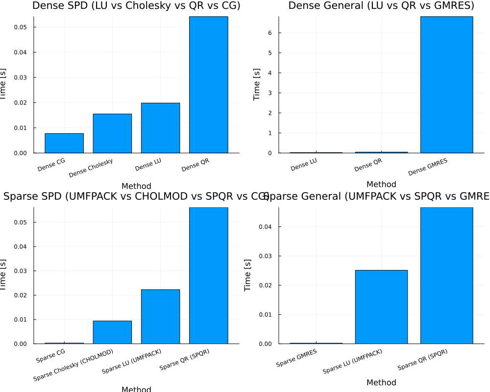
== Dense SPD ==
Dict("Dense LU" => 0.019838869000000002, "Dense Cholesky" => 0.015498259, "Dense QR" => 0.054151883000000005, "Dense CG" => 0.007737636000000001)
== Dense General ==
Dict("Dense LU" => 0.020005132000000002, "Dense GMRES" => 6.808577896, "Dense QR" => 0.045918054)
== Sparse SPD ==
Dict("Sparse CG" => 0.00030027, "Sparse QR (SPQR)" => 0.056110417, "Sparse LU (UMFPACK)" => 0.022294554, "Sparse Cholesky (CHOLMOD)" => 0.009384804)
== Sparse General ==
Dict("Sparse QR (SPQR)" => 0.046608782, "Sparse GMRES" => 0.00022120200000000001, "Sparse LU (UMFPACK)" => 0.025121761000000003)
Larger Matrix with OMP_NUM_THREADS=4
main(n_dense=2000, n_sparse=10_000, nrhs=4)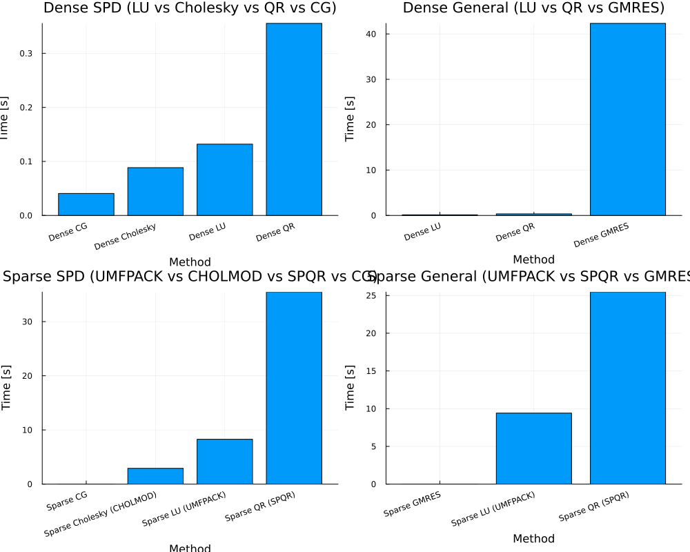
== Dense SPD ==
Dict("Dense LU" => 0.131976101, "Dense Cholesky" => 0.088446124, "Dense QR" => 0.355455481, "Dense CG" => 0.040695053)
== Dense General ==
Dict("Dense LU" => 0.132976766, "Dense GMRES" => 42.327230856, "Dense QR" => 0.345831791)
== Sparse SPD ==
Dict("Sparse CG" => 0.0034054370000000003, "Sparse QR (SPQR)" => 35.455767219, "Sparse LU (UMFPACK)" => 8.276840417, "Sparse Cholesky (CHOLMOD)" => 2.91287564)
== Sparse General ==
Dict("Sparse QR (SPQR)" => 25.457084755, "Sparse GMRES" => 0.0029985750000000003, "Sparse LU (UMFPACK)" => 9.414834372000001)
Larger Matrix with OMP_NUM_THREADS=8
main(n_dense=2000, n_sparse=10_000, nrhs=4)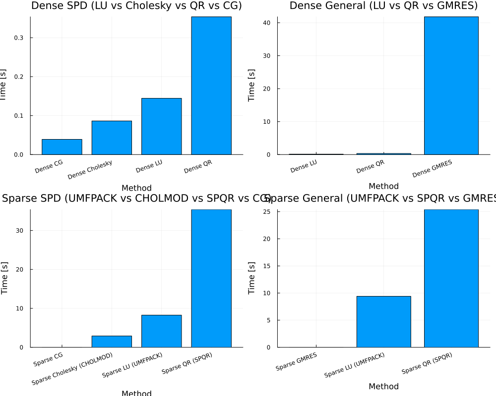
== Dense SPD ==
Dict("Dense LU" => 0.144481152, "Dense Cholesky" => 0.086386635, "Dense QR" => 0.35370767000000003, "Dense CG" => 0.039044995)
== Dense General ==
Dict("Dense LU" => 0.13258581900000002, "Dense GMRES" => 41.806955398, "Dense QR" => 0.33160050700000004)
== Sparse SPD ==
Dict("Sparse CG" => 0.0037104190000000004, "Sparse QR (SPQR)" => 35.388893107, "Sparse LU (UMFPACK)" => 8.261735826, "Sparse Cholesky (CHOLMOD)" => 2.90503845)
== Sparse General ==
Dict("Sparse QR (SPQR)" => 25.398382654000002, "Sparse GMRES" => 0.0029772450000000003, "Sparse LU (UMFPACK)" => 9.400900432)
GKS: cannot open display - headless operation mode active
BLAS.set_num_threads(8)
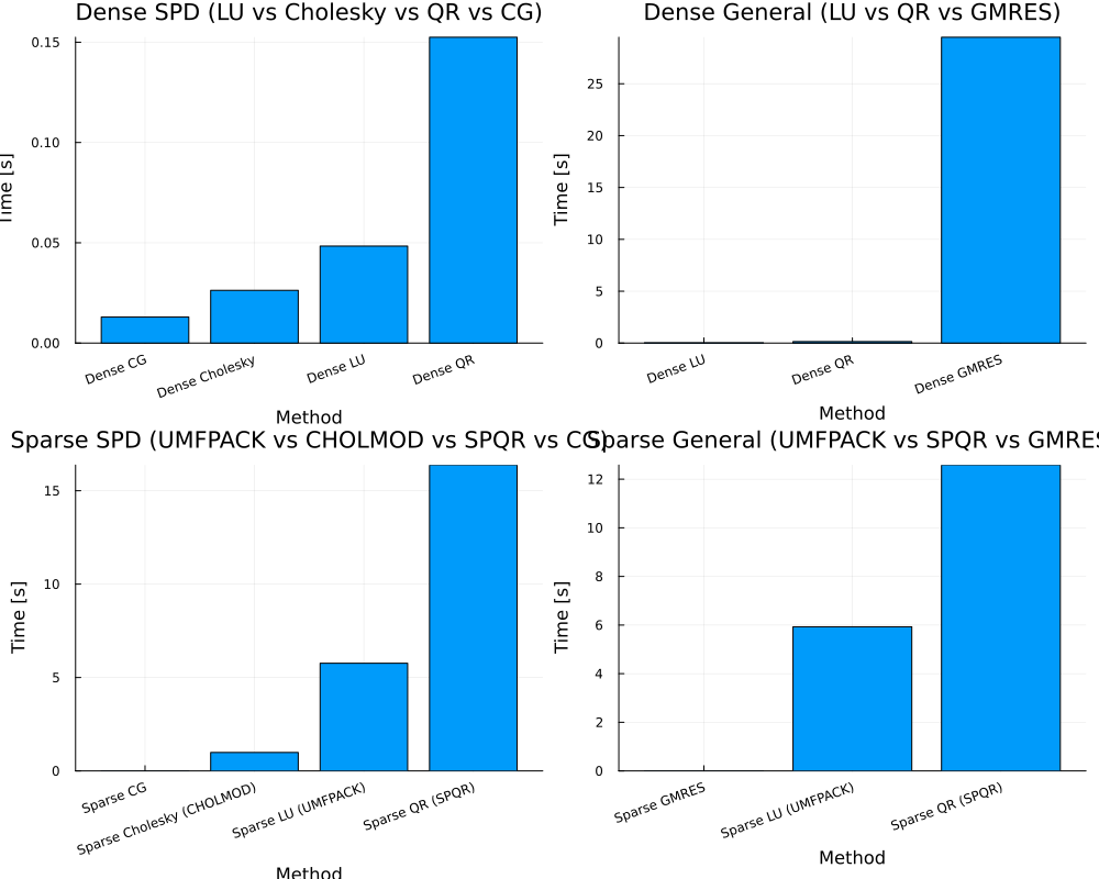
== Dense SPD ==
Dict("Dense LU" => 0.048364301000000005, "Dense Cholesky" => 0.026323567000000003, "Dense QR" => 0.152484221, "Dense CG" => 0.012993052000000001)
== Dense General ==
Dict("Dense LU" => 0.033466891000000006, "Dense GMRES" => 29.481741278, "Dense QR" => 0.14370575100000002)
== Sparse SPD ==
Dict("Sparse CG" => 0.003453944, "Sparse QR (SPQR)" => 16.374149409, "Sparse LU (UMFPACK)" => 5.762659557, "Sparse Cholesky (CHOLMOD)" => 0.986798601)
== Sparse General ==
Dict("Sparse QR (SPQR)" => 12.581917447, "Sparse GMRES" => 0.002984946, "Sparse LU (UMFPACK)" => 5.930593402)
GKS: cannot open display - headless operation mode active
Future work?
Diagonal matrix is added to this example toy problem. So, it is a bit easier to solve this problem with iterative method such as CG or GMRES. In physics simulation such as structural analysis In general, the trait of the stiffness matrix is not like that. So, in small problem, direct method is used as solver, and iterative method with preconditioning should be chosen for large scale problem.
Therefore, I should test actual physics problem as linear equation and do benchmarking next.
Preconditioning?
To solve original problem Ax = b, matrix M for preconditioning is prepared.
M^{-1}Ax = M^{-1}bBy applying M \approx A, what is intended is to improve condition of M^{-1}A. There are some ways to choose matrix M.
1: Jacobi, SOR
2: ILU, ICC
3: AMG