Multi-Physics (Thermoelastic Coupling) with Unidirectional Coupling

About

There are three main approaches to solving thermoelastic coupling problems: Unidirectional coupling, Bidirectional coupling, and Loose coupling.
In this context, we deal with one-way coupling, where one field is solved first and its results are then passed to the other field.
In the case of thermoelastic analysis, the heat problem is solved first, and the resulting temperature distribution is then used as input for the structural analysis.

Heat Conduct Equation

Heat Diffusion (Conduct) Term

a(u, v) = \int_{\Omega} k \nabla u \cdot \nabla v  d\Omega \quad \Longleftrightarrow \quad -\nabla \cdot (k \nabla T)

Internal Heat Generation

l_Q(v) = \int_{\Omega} Q  v d\Omega \quad \Longleftrightarrow \quad +Q

Robin Boundary Condition

 k \frac{\partial T}{\partial n} = h (T - T_{\mathrm{env}})

\int_{\Gamma_h} h T  v  d\Gamma = \int_{\Gamma_h} h  T_{\mathrm{env}} v  d\Gamma

Heat Radiation (Robin BC, Boundary Integral)

a_h(u, v) = \int_{\Gamma_h} h  u v  d\Gamma \quad \Longleftrightarrow \quad +hT

Heat Exchange with Ambient Air (Robin BC, boundary integral)

l_h(v) = \int_{\Gamma_h} h  T_{\mathrm{env}}  v d\Gamma \quad \Longleftrightarrow \quad +hT_{\mathrm{env}}

Dirichlet Boundary Condition

T = T_{\mathrm{env}} \quad \text{on } \Gamma_D

Implementation with Scikit-fem

# Parameters
k = 10.0
h = 5.0
T_env = 300.0
T_src = T_env + 300.0


@skfem.BilinearForm
def heat_form(u, v, w):
    return w.k * dot(grad(u), grad(v))


@skfem.LinearForm
def heat_load(v, w):
    # w.Q = 0
    # without Internal heat generation
    return w.Q * v
    # return 0.0 * v


@skfem.BilinearForm
def robin_form(u, v, w):
    # Surface integral (heat radiation term)
    return h * u * v


@skfem.LinearForm
def robin_load(v, w):
    # Temperature difference from outside temperature
    return h * T_env * v


# T_dofs_top = T_basis.with_elements(lambda x: x[2] == z_len)
T_facets_top = mesh.facets_satisfying(lambda x: abs(x[2] - z_len) < 1e-9)
T_facet_basis_top = skfem.FacetBasis(mesh, element, facets=T_facets_top)
T_dofs_bottom = T_basis.get_dofs(lambda x: x[2] == 0.0)
T_A = skfem.asm(heat_form, T_basis, k=k)
T_b = skfem.asm(heat_load, T_basis, Q=0.0)
T_A += skfem.asm(robin_form, T_facet_basis_top, h=h)
T_b += skfem.asm(robin_load, T_facet_basis_top, h=h, T_env=T_env)

T_sol = skfem.solve(
    *skfem.condense(
        T_A, T_b, D=T_dofs_bottom, x=np.full(T_dofs_bottom.N, T_src)
    )
)

print("Computed temperature range:", T_sol.min(), "→", T_sol.max())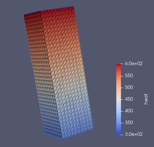

Structural Analysis with Temperature Distribution

Thermal Strain–induced Load

The stress–strain relationship (Hooke’s law) for a linear isotropic elastic material, including the effect of thermal strain due to a temperature change ΔT, can be expressed as follows:

\sigma = \lambda\mathrm{tr}(\varepsilon - \varepsilon_T)I + 2\mu(\varepsilon - \varepsilon_T)\\
where\space ε_T​=\alpha \Delta T I

\alpha is linear thermal expansion coefficient, and ε_T is isotropic thermal strain.

Substituting stress on Force equilibrium below,

-\nabla\cdot\sigma = 0

the following equation that depends on temperature is obtained.

-[\nabla\cdot(\lambda \mathrm{tr}(\varepsilon) I + 2\mu\varepsilon)
- \nabla\cdot\big((3\lambda + 2\mu)\alpha\Delta T I\big)] = 0

Implementation with Scikit-fem

E = 210e3
nu = 0.3
lam, mu = lame_parameters(E, nu)
T_std = 300.0
F_facet_ids = mesh.facets_satisfying(
    lambda x: np.isclose(x[2], z_len)
)
fbasis = skfem.FacetBasis(mesh, element, facets=F_facet_ids)
total_force = 100.0  # [N]


@skfem.Functional
def surface_measure(w):
    return 1.0


pressure = total_force / surface_measure.assemble(fbasis)


s_element = skfem.ElementVector(element)
s_basis = skfem.Basis(mesh, s_element)


@skfem.LinearForm
def l_comp(v, w):
    return pressure * dot(w.n, v)


@skfem.LinearForm
def thermal_load(v, w):
    ΔT = w.ΔT
    # return -3 * w.lam * w.alpha * ΔT * div(v)
    return -(3*w.lam + 2*w.mu) * w.alpha * ΔT * div(v)


ΔT_field = T_basis.interpolate(T_sol - T_std)
w = dict(alpha=1e-5, ΔT=ΔT_field, lam=lam, mu=mu)

s_A = linear_elasticity(lam, mu).assemble(s_basis)
s_b = skfem.asm(thermal_load, s_basis, **w)
s_b += l_comp.assemble(fbasis)
u = skfem.solve(*skfem.condense(s_A, s_b, D=s_basis.get_dofs()))