
Code
Pure-Python scikit-fem is highly flexible, stable, and very easy to work with. On the other hand, it may have limitations in terms of computation time. NGSolve, in contrast, is a library whose backend runs in C++, so it is expected to be faster. Its native implementation is also highly flexible. Therefore, we decided to compare the computation time and implementation characteristics of the two.
Implementation
Task I prepared
As a preliminary point, NGSolve is generally used by either importing mesh information and tags from an .msh file or generating meshes with Netgen and then solving the FEM problem. In this regard, its flexibility is somewhat limited, and I found it a bit difficult to work with. I attempted to manually define boundaries and other settings, but was unsuccessful.
In contrast, scikit-fem is highly flexible because it can import a mesh as long as the information can be loaded into a NumPy array. For a fair comparison, I generated an .msh file and compared the results under equivalent conditions.
Generate .msh
Generate 1 x 0.1 x 0.1 box with gmsh
import gmsh

gmsh.initialize()
gmsh.model.add("tension_bar")

L, W, H = 1.0, 0.1, 0.1
lc = 0.01

# --- ジオメトリ作成 ---
gmsh.model.occ.addBox(0, 0, 0, L, W, H)
gmsh.model.occ.synchronize()

# --- サイズ制御 ---
gmsh.option.setNumber("Mesh.CharacteristicLengthMin", lc)
gmsh.option.setNumber("Mesh.CharacteristicLengthMax", lc)

# --- 物理グループ設定 ---
eps = 1e-8  # 少し幅を持たせるのがミソ

# dim=2 の面を、座標で拾う(← ここを occ ではなく model 側から)
left = gmsh.model.getEntitiesInBoundingBox(-eps, 0, 0,
                                           eps,  W, H, dim=2)
gmsh.model.addPhysicalGroup(2, [s[1] for s in left], tag=1)
gmsh.model.setPhysicalName(2, 1, "left")

right = gmsh.model.getEntitiesInBoundingBox(L - eps, 0, 0,
                                            L + eps, W, H, dim=2)
gmsh.model.addPhysicalGroup(2, [s[1] for s in right], tag=2)
gmsh.model.setPhysicalName(2, 2, "right")

# 体積
vol = gmsh.model.getEntities(dim=3)
gmsh.model.addPhysicalGroup(3, [vol[0][1]], tag=10)
gmsh.model.setPhysicalName(3, 10, "bar")

# --- メッシュ生成 & 書き出し ---
gmsh.option.setNumber("Mesh.SaveAll", 1)        # 念のため全部出す
gmsh.option.setNumber("Mesh.MshFileVersion", 2.2)
gmsh.model.mesh.generate(3)
gmsh.write("tension_bar.msh")

gmsh.finalize()
print("✅ Saved: tension_bar.msh")
import time
import numpy as np
import skfem as sk


def run_skfem(mesh_file: str):
    from skfem.models.elasticity import lame_parameters
    from skfem.models.elasticity import linear_elasticity
    from skfem.helpers import dot

    E, nu = 210e3, 0.3
    traction_value = 1e-3
    lam, mu = lame_parameters(E, nu)

    t0_total = time.perf_counter()
    mesh = sk.MeshTet.load(mesh_file)
    basis = sk.Basis(mesh, sk.ElementVector(sk.ElementTetP1()))
    print(f"mesh.p {mesh.p.shape}")

    # @sk.BilinearForm
    # def elasticity(u, v, w):
    #     eps_u, eps_v = sk.sym_grad(u), sk.sym_grad(v)
    #     return lam * sk.trace(eps_u) * sk.trace(eps_v) + 2 * mu * sk.ddot(eps_u, eps_v)

    @sk.LinearForm
    def traction(v, w):
        return traction_value * dot(np.array([1, 0, 0]), v)

    left = mesh.facets_satisfying(lambda x: np.isclose(x[0], 0))
    right = mesh.facets_satisfying(lambda x: np.isclose(x[0], 1.0))
    fixed = basis.get_dofs(facets=left).all()
    fbasis = sk.FacetBasis(
        mesh, sk.ElementVector(sk.ElementTetP1()), facets=right
    )

    # アセンブリ
    t0 = time.perf_counter()
    # K = sk.asm(elasticity, basis)
    K = linear_elasticity(lam, mu).assemble(basis)
    F = sk.asm(traction, fbasis)
    t_asm = time.perf_counter() - t0

    # Dirichlet条件 + 解く
    K, F = sk.enforce(K, F, D=fixed)
    t1 = time.perf_counter()
    u = sk.solve(K, F)
    t_solve = time.perf_counter() - t1

    t_total = time.perf_counter() - t0_total

    print(f"[scikit-fem] Total: {t_total:.3f}s | Assembly: {t_asm:.3f}s | Solve: {t_solve:.3f}s | max|u|={np.abs(u).max():.3e}")
    return mesh.p.T, u.reshape(-1, 3), [t_total, t_asm, t_solve]


def run_ngsolve(mesh_file: str):
    import time
    import numpy as np
    from ngsolve import (
        Mesh, VectorH1, BilinearForm, LinearForm, GridFunction,
        CoefficientFunction, grad, Trace, Id, InnerProduct,
        dx, ds, x, IfPos,
    )
    from netgen.read_gmsh import ReadGmsh

    # --- 材料・荷重パラメータ ---
    E, nu = 210e3, 0.3
    traction_value = 1e-3
    lam = E * nu / ((1 + nu) * (1 - 2 * nu))
    mu = E / (2 * (1 + nu))

    t0_total = time.perf_counter()

    # --- メッシュ読み込み (.msh) ---
    ngmesh = ReadGmsh(mesh_file)
    mesh = Mesh(ngmesh)
    print(f"nv = {mesh.nv}")

    # --- x のレンジを自動取得 ---
    xs = [vtx.point[0] for vtx in mesh.vertices]
    xmin, xmax = min(xs), max(xs)
    print(f"x-range: [{xmin:.6g}, {xmax:.6g}]")

    # Dirichlet は座標で後から指定するので、ここでは dirichlet="" は指定しない
    fes = VectorH1(mesh, order=1)

    u = fes.TrialFunction()
    v = fes.TestFunction()

    # --- 線形弾性の弱形式 ---
    def eps(w):
        return 0.5 * (grad(w) + grad(w).trans)

    def sigma(w):
        return lam * Trace(eps(w)) * Id(3) + 2 * mu * eps(w)

    a = BilinearForm(fes, symmetric=True)
    a += InnerProduct(sigma(u), grad(v)) * dx

    # --- Neumann: x ≈ xmax の面だけに traction をかける ---
    eps_coord = 1e-8 * max(1.0, abs(xmax - xmin))  # スケールに合わせて少しだけ幅を取る
    # x > xmax - eps のとき 1、それ以外 0
    indicator_right = IfPos(x - (xmax - eps_coord), 1.0, 0.0)

    tvec = CoefficientFunction((traction_value, 0.0, 0.0))
    f = LinearForm(fes)
    # 「すべての境界 ds」に対して、x≃xmax のところだけ traction が効く
    f += InnerProduct(indicator_right * tvec, v) * ds

    # --- アセンブリ ---
    t0 = time.perf_counter()
    a.Assemble()
    f.Assemble()
    t_asm = time.perf_counter() - t0

    print("||f|| =", f.vec.Norm())  # 荷重がちゃんと入っているか確認用

    # --- GridFunction と FreeDofs(BitArray コピー) ---
    gfu = GridFunction(fes)

    freedofs0 = fes.FreeDofs()             # BitArray
    freedofs = type(freedofs0)(freedofs0)  # 古い NGSolve 向けコピー

    # --- Dirichlet: x ≈ xmin の頂点の DoF を拘束 & 0 固定 ---
    for vtx in mesh.vertices:
        if abs(vtx.point[0] - xmin) < eps_coord:
            dnums = fes.GetDofNrs(vtx)  # この頂点に対応する DoF 番号
            for d in dnums:
                freedofs[d] = False   # 拘束
                gfu.vec[d] = 0.0      # Dirichlet 値

    # --- 解く ---
    t1 = time.perf_counter()
    gfu.vec.data = a.mat.Inverse(freedofs, inverse="sparsecholesky") * f.vec
    t_solve = time.perf_counter() - t1

    t_total = time.perf_counter() - t0_total

    # --- 頂点座標と変位を numpy 配列に ---
    coords = np.zeros((mesh.nv, 3))
    u_vals = np.zeros((mesh.nv, 3))

    for i, vtx in enumerate(mesh.vertices):
        p = vtx.point
        x0, y0, z0 = p[0], p[1], p[2]
        coords[i, :] = (x0, y0, z0)

        # MeshPoint を通して点評価
        val = gfu(mesh(x0, y0, z0))
        u_vals[i, :] = np.array(val)

    print(
        f"[NGSolve] Total: {t_total:.3f}s | "
        f"Assembly: {t_asm:.3f}s | "
        f"Solve: {t_solve:.3f}s | "
        f"max|u|={np.max(np.abs(u_vals)):.3e}"
    )

    return coords, u_vals, [t_total, t_asm, t_solve]


def visualize(
    skfem_times, ngsolve_times,
    dst_path: str = "benchmark_comparison.png"
):
    import matplotlib.pyplot as plt
    import numpy as np

    # データ(あなたの測定結果)
    labels = ["Total", "Assembly", "Solve"]

    x = np.arange(len(labels))  # X軸位置
    width = 0.35                # 棒の幅

    fig, ax = plt.subplots(figsize=(6, 4))
    rects1 = ax.bar(x - width/2, skfem_times, width, label='scikit-fem', color='#4C72B0')
    rects2 = ax.bar(x + width/2, ngsolve_times, width, label='ngsolve', color='#55A868')

    # 軸ラベル・タイトル
    ax.set_ylabel('Time [s]')
    ax.set_title('FEM Benchmark Comparison')
    ax.set_xticks(x)
    ax.set_xticklabels(labels)
    ax.legend()

    # 各棒に値を表示
    def autolabel(rects):
        for rect in rects:
            height = rect.get_height()
            ax.annotate(f'{height:.2f}',
                        xy=(rect.get_x() + rect.get_width() / 2, height),
                        xytext=(0, 3),
                        textcoords="offset points",
                        ha='center', va='bottom', fontsize=9)

    autolabel(rects1)
    autolabel(rects2)

    fig.tight_layout()
    plt.savefig(dst_path, dpi=200)
    # plt.show()

    print("✅ Saved: benchmark_comparison.png")


def compare_displacements(coords1, u1, coords2, u2, tol=1e-8):
    # 両メッシュが一致する前提
    assert np.allclose(coords1, coords2, atol=tol)

    diff = u1 - u2
    abs_err = np.linalg.norm(diff, axis=1)
    l2_err = np.linalg.norm(abs_err)
    rel_err = l2_err / np.linalg.norm(np.linalg.norm(u1, axis=1))
    max_err = np.max(abs_err)

    print(f"‣ L2 error = {l2_err:.3e}")
    print(f"‣ Relative L2 error = {rel_err:.3e}")
    print(f"‣ Max abs error = {max_err:.3e}")


if __name__ == "__main__":
    msh = "tension_bar.msh"  # Gmshで生成済みメッシュ

    print("run_skfem")
    skfem_coords, skfem_disp, skfem_times = run_skfem(msh)

    print("run_ngsolve")
    ngsolve_coords, ngsolve_disp, ngsolve_times = run_ngsolve(msh)
    tT_s, tA_s, tS_s = skfem_times
    tT_m, tA_m, tS_m = ngsolve_times

    print("skfem max|u| =", np.abs(skfem_disp).max())
    print("ngsolve  max|u| =", np.abs(ngsolve_disp).max())
    print("ratio (skfem/ngsolve) ≈", np.abs(skfem_disp).max() / np.abs(ngsolve_disp).max())

    compare_displacements(skfem_coords, skfem_disp, ngsolve_coords, ngsolve_disp)

    print("\n=== Benchmark Summary ===")
    print(f"scikit-fem: Total {tT_s:.3f}s | Assembly {tA_s:.3f}s | Solve {tS_s:.3f}s")
    print(f"ngsolve:       Total {tT_m:.3f}s | Assembly {tA_m:.3f}s | Solve {tS_m:.3f}s")

    visualize(
        skfem_times, ngsolve_times,
    )
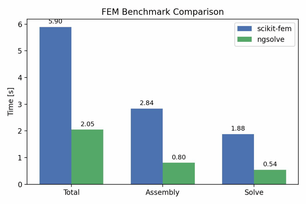
Result
Ngsolve is x3 faster.
run_skfem

mesh.p (3, 10350)
[scikit-fem] Total: 5.895s | Assembly: 2.835s | Solve: 1.881s | max|u|=4.745e-09
run_ngsolve

WARNING: Physical groups detected - Be sure to define them for every geometrical entity.
nv = 10350
x-range: [0, 1]
||f|| = 8.958356960396356e-07
[NGSolve] Total: 2.050s | Assembly: 0.804s | Solve: 0.542s | max|u|=5.068e-09
skfem max|u| = 4.745188501650329e-09
ngsolve  max|u| = 5.068472451718415e-09
ratio (skfem/ngsolve) ≈ 0.9362166899104917
‣ L2 error = 1.708e-08
‣ Relative L2 error = 6.109e-02
‣ Max abs error = 3.740e-10

=== Benchmark Summary ===
scikit-fem: Total 5.895s | Assembly 2.835s | Solve 1.881s
ngsolve:       Total 2.050s | Assembly 0.804s | Solve 0.542s
✅ Saved: benchmark_comparison.png