Cantilever Task with Gridap / FluxFEM
In previous articles, nonlinear structural analysis (cantilever) is solved with Gridap and FluxFEM. As you can see, the both result represent same results. It means that both computation results are reliable. At least both implementation use same formulation with weak-form.
In this article, I did some experiments and did benchmark to show which points in both framework are valuable.
Abstract / Motivation
The main motivation of this study is to determine how far FluxFEM/JAX can reuse compilation across meshes of different sizes, and to clarify where its practical limits arise. Gridap appeared to benefit strongly from same-session warm-run reuse even when the mesh changed, so it became necessary to compare the shape-sensitive JAX/XLA compilation model against the more flexible reuse behavior observed in Julia/Gridap. In particular, the goal was to separate runtime differences caused by compilation effects from those caused by assembly and linear-solver costs when the mesh size changes.
A second motivation was to clarify the actual value proposition of FluxFEM. If FluxFEM were substantially
worse than Gridap in forward-solve runtime alone, then positioning it as a pure nonlinear FEM solver would be difficult. On the other hand, FluxFEM offers a different advantage through JAX-based automatic
differentiation, allowing constitutive laws, residuals, and Jacobians to remain differentiable within a
unified workflow. For that reason, this study did not stop at comparing total wall times; it explicitly
decomposed compile-like overhead, steady-state warm-run cost, assembly-like cost, and the effect of the
linear-solver backend. The broader aim was to determine whether FluxFEM’s weaknesses come primarily from Python/JAX itself, or from solver-backend choices and execution structure.
Experimental Setup
This study compares Gridap and FluxFEM on a 3D Neo-Hookean tensile bar benchmark. Three meshes were used: tension_bar_lc3_0.msh, tension_bar_lc2_0.msh, and tension_bar_lc1_5.msh, and same-session warm-run experiments were carried out in this order from coarse to fine. The loading condition was a uniform surface traction (0, 0.01, 0) on the right boundary with the left boundary fully fixed. The number of load steps was 20 for the main warm-run experiments and 5 for the isolated compile-proxy experiments. In all cases, the nonlinear solve used Newton’s method with line search enabled.
On the FluxFEM side, two linear-solver backends were tested: spsolve and petsc_shell. On the Gridap side, the focus was on reuse within a single Julia session. In addition to total wall time, FluxFEM recorded linear
solve, initial Jacobian, initial residual, residual eval, and control/other, while Gridap recorded assembly,
solve, first_step, and remaining_steps_avg. To reduce the influence of first-run effects, isolated runs were
also executed for each mesh independently. For Gridap, one extra warmup solve was inserted, and a compile-oriented proxy was defined as compile_only_proxy = warmup_solve_s – remaining_steps_avg_s. Therefore, the “compile time” reported here is not a strict pure compilation time, but a proxy that includes first-call JIT, initialization, and fixed startup overhead.
- tension_bar_lc3_0.msh: 726 nodes → 2178 total DoFs
- tension_bar_lc2_0.msh: 1742 nodes → 5226 total DoFs
- tension_bar_lc1_5.msh: 3603 nodes → 10809 total DoFs
Result
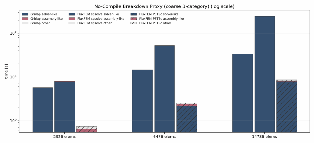
Total Computational Cost for Assembly + Solve + others excluding compile
The Total Cost for Assembly + Solve + others excluding compile comparison shows that, even in steady state, FluxFEM’s performance depends very strongly on the choice of linear-solver backend. In particular, when using spsolve, the total cost grows rapidly as the mesh becomes finer, and most of the steady-state runtime becomes dominated by the linear solve. In contrast, when petsc_shell is used, the total cost improves substantially and, under the present benchmark conditions, becomes much closer to Gridap. Therefore, it is not accurate to conclude that FluxFEM is slow simply because it is based on Python/JAX; a large portion of the compile-removed total-cost gap is actually explained by the linear-solver backend.
This result is also important for clarifying the deeper difference between Gridap and FluxFEM. Gridap not only reuses cold-start compilation effectively, but also shows consistently strong steady-state total runtime. FluxFEM, by contrast, changes character significantly depending on the solver backend. With spsolve, it appears clearly disadvantaged as a forward-solve engine, whereas with PETSc it improves to a level that is no longer catastrophically worse in practical terms. For that reason, the value of FluxFEM should not be judged only by total warm-run time; it must also be evaluated in terms of which backend produces that cost, and how the system supports a broader AD-enabled research workflow.
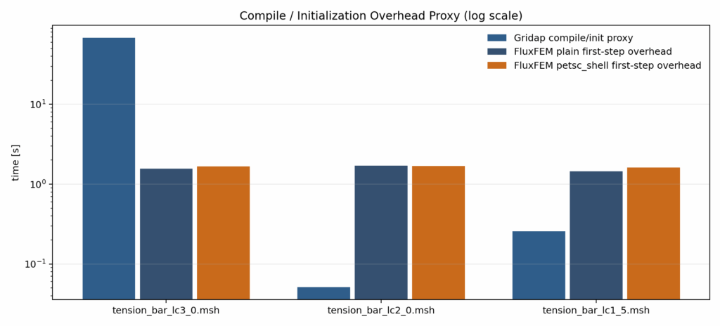
Computational Cost for Compiling
This bar plot compares a compile-oriented proxy rather than a strict pure compilation time. The key point is that the large compile-like overhead in Gridap is concentrated in the first cold-session run, while the
overhead becomes much smaller in subsequent runs. This reduction occurs because the first solve! triggers Julia method specialization and JIT compilation across the nonlinear solver stack, element integration, assembly, and the linear-solver path, and the resulting compiled code is retained within the same session. Therefore, Gridap’s advantage is not that compilation is always cheap, but that the large initial JIT cost can be reused very effectively once it has been paid. By contrast, the corresponding proxy remains relatively small for FluxFEM across all tested meshes, indicating that FluxFEM’s main limitation is not pure compilation cost itself but the cost structure that remains in steady-state execution. This bar plot focuses on assembly-oriented runtime after removing as much first-run compile-related overhead as possible. It shows that Gridap’s overall warm-run advantage should not be interpreted simply as overwhelming superiority in steady-state assembly cost alone. Once compile-like effects are reduced, the remaining assembly-oriented cost does not always separate Gridap and FluxFEM by a large margin. This suggests that Gridap’s strong same-session behavior is driven not only by runtime efficiency but also by very effective reuse of the initial compilation cost. At the same time, this comparison should be read as a diagnostic approximation rather than a perfectly matched assembly-time measurement, since the assembly-oriented terms are defined differently on the two sides. Even so, the result makes clear that FluxFEM’s disadvantage cannot be reduced to “slow Python/JAX assembly,” and that the solver backend and the broader steady-state runtime structure must be considered separately.
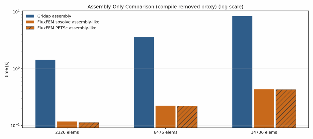
Computational Cost for Assembling with warm-start
The main takeaway from the assembly only nocompile comparison is that Gridap’s advantage should not be interpreted simply as “its numerical execution is always overwhelmingly faster.” This figure was introduced to remove as much first-run compile-related overhead as possible and to focus on steady-state, assembly-oriented cost. Under that view, Gridap still benefits strongly from cold-start compile reuse, but once compilation effects are reduced, its assembly-like runtime does not always dominate FluxFEM by a large margin. This suggests that Gridap’s strength in same-session warm-run performance is not explained solely by superior steady-state assembly throughput, but also by its ability to reuse the initial JIT cost very effectively. At the same time, this comparison is not a strict apples-to-apples measurement and should be interpreted carefully. On the Gridap side, assembly is a coarse indicator centered on FEOperator construction and related setup, whereas on the FluxFEM side, the assembly-like term is based mainly on residual evaluation. Therefore, the figure should not be read as a perfectly matched assembly-time comparison, but rather as a diagnostic view of how much assembly-oriented cost remains once the linear solve is no longer the dominant term. Even with that limitation, the result is still useful: it shows that FluxFEM’s disadvantage cannot be attributed entirely to slow Python/JAX assembly, and that solver backend choice and steady-state solve cost must be analyzed separately.
Why is FluxFEM not flexible?
FluxFEM requires recompilation when shapes differ because the underlying JAX/XLA compilation model is strongly dependent on array shape and dtype. In finite-element computations, changing the mesh changes quantities such as the number of elements n_elems, the number of global degrees of freedom n_dofs, sparse data lengths, and the sizes of gather/scatter operations. Since FluxFEM handles these shape-sensitive arrays throughout residual evaluation, Jacobian construction, and global assembly, a change in mesh size is often seen by JAX as a different computation graph. As a result, an existing compiled artifact cannot always be reused directly, and retracing/recompilation is likely to occur. This is a major contrast with Gridap/Julia, where reuse is driven more naturally by type structure than by exact array shapes.
To address this issue, several strategies were explored and implemented in FluxFEM in order to improve compile reuse. The first was a bucket/padding strategy, in which different meshes were rounded up to a shared shape so that the same compilation cache could be reused. However, this approach introduced substantial padding overhead for coarse meshes and often worsened runtime. The second was the fixed_chunk_tail strategy, which does not attempt to make the entire global shape identical, but instead reuses fixed-size chunk kernels while processing only the final remainder in a separate path. This removed the need for large padding, although the cost of chunk orchestration still remained. The overall conclusion is that, within JAX, it is difficult to achieve Gridap-like behavior in which a single compiled global solve is fully reused across arbitrary shapes. A more realistic strategy is therefore to maximize compile reuse at the level of local kernels or fixed-size chunks rather than at the level of the entire global assembly.
Conclusion
From these experiments, the value of Gridap can be concluded to lie primarily in its strength as a forward-
solve engine. In particular, under same-session warm-run conditions, it can reuse the initial cold-start JIT
very effectively, allowing it to maintain high efficiency even when the mesh size changes. This shows that
Julia/Gridap’s flexible compile reuse has clear practical value for nonlinear FEM solving. Therefore, for
workloads that require many stable and efficient forward simulations, Gridap is a highly attractive choice.
By contrast, the value of FluxFEM does not primarily lie in pure forward-solve speed. In the present
comparison, especially along the spsolve path, it is disadvantaged relative to Gridap, and it does not exhibit the same natural warm-run flexibility across changing meshes. However, FluxFEM has a fundamentally different strength: constitutive laws, residuals, and Jacobians remain differentiable within a unified JAX/AD workflow. In addition, with petsc_shell, its steady-state runtime improves significantly, so it should not be regarded as unusable as a forward solver. The most appropriate conclusion, therefore, is that FluxFEM should not be positioned as a framework whose main goal is to outperform Gridap as a solver, but rather as a Python-native differentiable FEM workflow built around automatic differentiation.
Business Perspective
The significance of building FluxFEM on top of JAX is not limited to automatic differentiation alone. JAX is a general-purpose foundation that naturally connects finite-element computation not only to scientific
computing, but also to deep learning, optimization, inverse problems, generative models, and surrogate
modeling. This means that a FEM solver does not have to remain an isolated piece of domain-specific code; instead, it can be integrated into a broader Python-based workflow that includes machine learning and data-driven model development. In this sense, the value of FluxFEM is not only in solver capability itself, but also in the fact that JAX provides a shared computational substrate through which ideas and tools from other modeling communities can be brought into FEM more easily.
Even more importantly, this choice can reduce development cost at the community level. If the FEM community must maintain a separate differentiation stack, a separate GPU backend, a separate optimization workflow, and a separate infrastructure for model development, then the costs of maintenance, education, and collaboration become much higher. By contrast, using JAX makes it possible for researchers in machine learning, numerical methods, and applied computational science to share a common set of abstractions: array programming, AD, JIT compilation, and the broader Python ecosystem. This matters independently of whether a single FEM solver is the absolute fastest. It creates value by improving code sharing, reuse, collaboration, and integration of experimental workflows, thereby lowering the overall cost of development across the broader community.
Appendix.
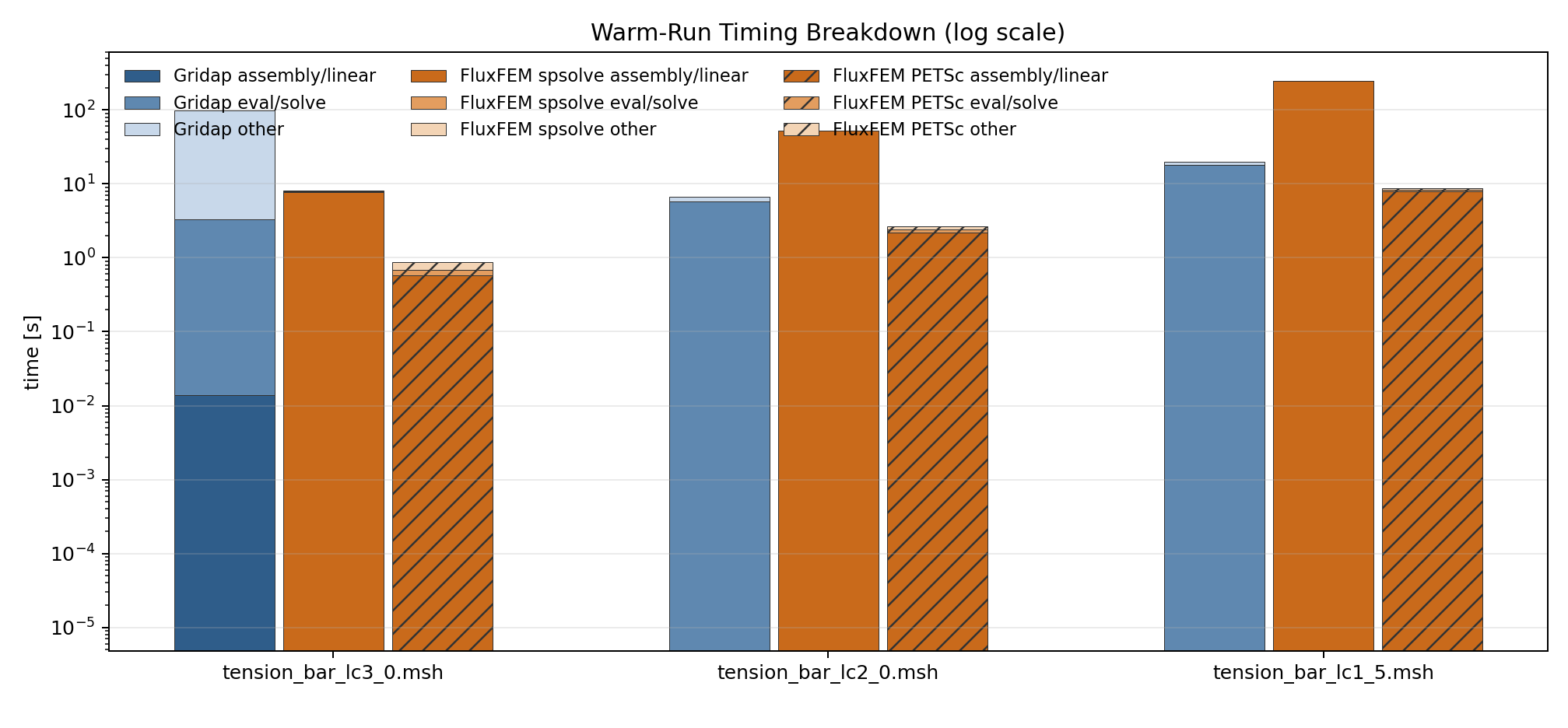
Total Computational Cost Breakdown including compile
Note that compile is run on the first step (tension_bar_lc3_0.sh). This is why computation time for this mesh is greater than following meshes

Total Computational Cost Breakdown excluding compile
