EfficientAD
https://arxiv.org/abs/2303.14535
What authors claim
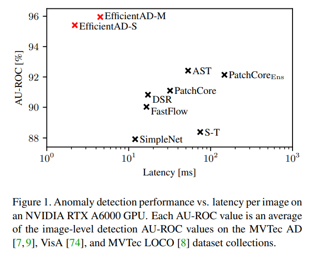
They claim to have achieved State of the Art in the task of learning solely from normal images and detecting anomalies. Furthermore, as shown in Figure 1 of the paper, it is reported to be a model that performs very well not only in detection performance but also in terms of computational speed.
My Perspective
In this paper, they present a model that achieves exceptionally high anomaly detection performance at the pixel-level using a quite simple convolutional neural network. In my personal opinion, the contribution of this paper is that it lies in effectively leveraging the specificity of the anomaly detection task. That is, while the subject of being trained itself is very simple and does not require complex neural networks, on the other hand, it necessitates a successful definition of anomalies and careful control of the learning targets and data. Consequently, the network architecture is quite simple, but the learning scheme appears somewhat specialized. In this paper, I believe that anomalies are well-defined through distillation and the penalty term created from natural images from the ImageNet dataset. Additionally, by detecting local anomalies and global anomalies through separate approaches, it accommodates various types of anomaly detection tasks.
This approach demonstrates exceptionally high anomaly detection capability, and it may signal the culmination of the evaluation phase on the MVTech dataset.
What’s important, as is natural, is understanding whether your dataset is suitable for this approach and using it accordingly. Especially in tasks like anomaly detection, in order to achieve good performance, you need to build the model with some strong assumptions, so it is crucial to understand what kind of computations are being performed. In this way, it’s not clear whether this approach is suitable for your dataset, but the fact that the computation time is very short is undoubtedly an advantage.
Architechture
I believe that it’s easier to understand by grasping the overall picture rather than delving into the finer technical details of the proposed method or the evolution of related work, as presented in the paper. (In addition to this point, I am not familiar with the history). Therefore, I will explain it starting from the overall flow and how anomalies are extracted.
How to Extract Anomaly Masks
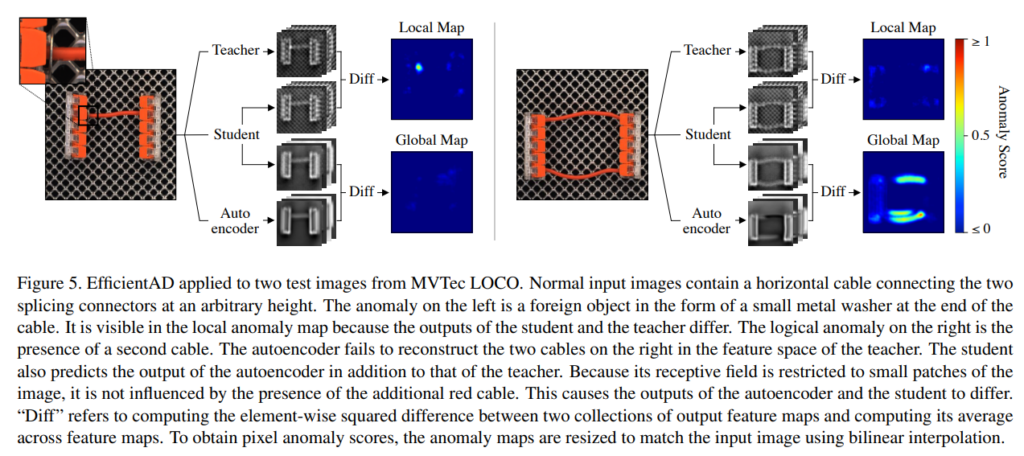
As shown in Figure 5 of the paper, this method employs three neural networks to detect anomalies.
- Teacher Network
- Student Network
- Auto Encoder
Both the Teacher Network and the Student Network have essentially the same structure, and the outputs obtained from their final layers are images. However, the Student Network has twice the number of channels compared to the Teacher Network. The output feature map obtained from the Auto Encoder is the same as that of the Teacher Network. In this method, anomalies are detected by taking the difference between the outputs obtained from these networks.
- Difference between the outputs of the Teacher Network and the Student Network
- Anomalies are learned to be detected based on local features in this difference (Figure 5, right in the paper).
- Difference between the outputs of the Student Network and the Auto Encoder
- Anomalies are learned to be detected based on band features in this difference (Figure 5, left in the paper).
Anomaly detection is peformed by averaging both anomaly map.
What do these Neural Networks learn? What kind of Loss functions are used?
Teacher Network Pre-Training
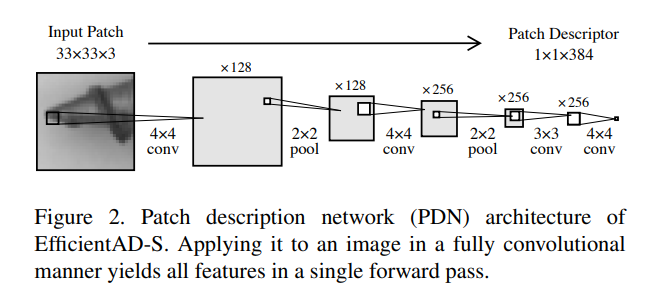
The Teacher Network is trained by distilling knowledge from WideResNet-101, which has been trained on ImageNet. The loss function is defined as the mean squared error between the outputs of WideResNet-101 and the Teacher Network when presented with images from ImageNet as input. The Teacher Network (and Student Network also) consists of an extremely simple 4-layer convolutional structure called PDN, Figure 2 represents the network architecture of PDN. As you can see, it is extremely simple and functions as a local feature extractor with a receptive field of 33×33 patches. And it can compute on a 256×256 image in under 800 µs (when using an NVIDIA RTX A6000 GPU).
In other words, the Teacher Network is learning basic/general features.
Student Network Training from Teacher
Next, let’s discuss the learning process of the Student Network, which naturally learns from the Teacher Network. However, there’s a clever twist. The Student Network learns the mean squared error with the output of the Teacher Network, but it only learns from specific pixels that meet certain conditions. The condition is that there is a difference greater than a certain threshold. This threshold is determined by percentiles of all pixels. so-called “Quantile”. The “Quantile” is set to 0.999 on their setting. They refer to this loss as the “hard feature loss.” This loss function appears to contribute to reducing false negatives. As shown in Figure 4, this loss might have the potential to suppress overfitting to easily learnable backgrounds.
\begin{align}
D(C, H, W)=(CHW)^{-1}\displaystyle\sum_{C,H,W} \begin{Vmatrix}
  T(I)_C - S(I)_C
\end{Vmatrix}^2 \\
L_{hard}=D(C, H, W) [D(C, H, W)>p_{hard}]\\
L_{ST}=L_{hard}+\displaystyle\sum_{C,H,W} \begin{Vmatrix}
  S(P)_C
\end{Vmatrix}^2_F
\end{align}\\

p_{hard}=0.999
T: Teacher Network
S: Student Network
P: images from pretrain dataset (like ImageNet)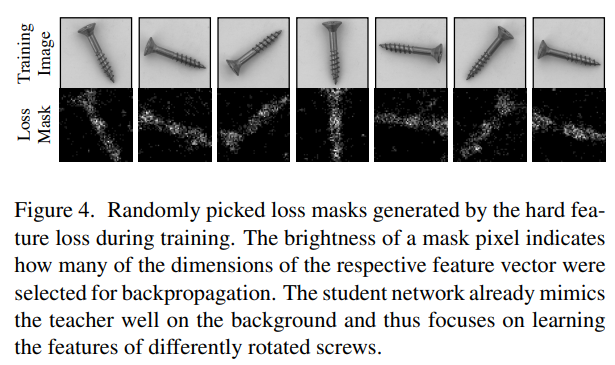
Penalty Term to Student Network
A penalty term is applied to the Student Network. This term is designed to make the output of the Student Network, when given the same images (natural images) used by the Teacher Network for pretraining, approach zero. In their case, they randomly select and utilize images from the ImageNet dataset for this purpose. They say that “This penalty hinders the student from generalizing its imitation of the teacher to out-of-distribution images”.
Logical Anomaly Detection
They say that “There are many types of logical anomalies, such as missing, misplaced, or surplus objects or the violation of geometrical constraints, for example, the length of a screw” and this sort of “logical anomaly” should be detected by using AutoEncoder. They probably mean that they want to detect anomalies in the global feature space, which cannot be determined solely from local features.
Therefore, the Teacher Network serves as the teacher, and the autoencoder is trained.
\begin{align}
L_{AE}=(CHW)^{-1}\displaystyle\sum_{C} \begin{Vmatrix}
  T(I)_C - A(I)_C
\end{Vmatrix}^2
\end{align}
A: AutoEncoderHowever, in practice, not only logical (global) anomalies but also normal images exhibit imperfect reconstructions, and autoencoders are known to struggle with reconstructing fine-grained patterns [1, 2]. Using the difference between the teacher’s output and the autoencoder’s reconstruction as an anomaly map is likely to result in a high occurrence of false positives.
\begin{align}
L_{AE}=(CHW)^{-1}\displaystyle\sum_{C} \begin{Vmatrix}
  A(I)_C - S'(I)_C
\end{Vmatrix}^2
\end{align}
S': Student Network - (2nd banch of channel output)Evaluation
For detection, evaluation was conducted using AU-ROC, and for segmentation, AU-PRO was used. These evaluations resulted in achieving state-of-the-art (SOTA) performance.
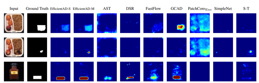
What’s interesting is that the Appendix compiles the anomaly output results of various methods. In the MVTech competition, the goal is to achieve good performance on various types of datasets. However, it’s not guaranteed that methods developed in such contexts will work well for your dataset. Viewing such figures might help you find an approach that fits your dataset.
Reference
[1]Paul Bergmann, Sindy Lowe, Michael Fauser, David Sattlegger, and Carsten Steger. Improving Unsupervised Defect Segmentation ¨ by Applying Structural Similarity to Autoencoders. In Proceedings of the 14th International Joint Conference on Computer Vision,Imaging and Computer Graphics Theory and Applications – Volume 5: VISAPP, pages 372–380. INSTICC, SciTePress, 2019
[2]Alexey Dosovitskiy and Thomas Brox. Generating Images with Perceptual Similarity Metrics based on Deep Networks. In Advances in Neural Information Processing Systems, pages 658–666, 2016. 5