Diagonalization of matrices plays a crucial role in numerical computations. However, when diagonalization of a matrix is not possible, how can we deal with the problem? A commonly used approach is a method called Jordan Canonical Form, which is a form of quasi diagonalization.
Jordan Blocks(Cell)
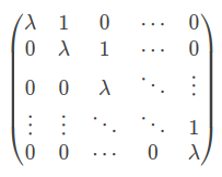
Let’s say we have a N by N Jordan Cell which eigenvalue is \lambda. It is denoted as
J_N(\lambda)=\begin{pmatrix}
\lambda & 1       & 0       & \cdots  & 0 \\
0       & \lambda & 1       & \cdots  & 0 \\
0       & 0       & \lambda & \ddots  & \vdots \\
\vdots  & \vdots  & \ddots  & \ddots  & 1 \\
0       & 0       & \cdots  & 0       & \lambda
\end{pmatrix}
Let’s see an example for our understanding. when it is \lmabda = 3, and block size = 2,
J_2(3) = \begin{pmatrix}
3 & 1 \\
0 & 3 \\
\end{pmatrix}
Theorem
Any square matrix ( A ) can be decomposed using an appropriate invertible matrix ( P ) and a Jordan canonical form (J) as follows.
P^{-1}A P = J = \begin{pmatrix}
J_{k_1}({\lambda_1}) &  &  & \\
 & J_{k_2}({\lambda_2}) &  & \\
 &  & \ddots & \\
 &  & & J_{k_n}({\lambda_n})\\
\end{pmatrix}
\lambda’s are eigenvalues of matrix A. What’s important is that the Jordan canonical form is unique up to the order of the Jordan blocks.
About
Here, J is the Jordan normal form of A. This transformation relies on finding the matrix P, which consists of the eigenvectors and generalized eigenvectors of A as its columns. This process is generally complex, especially for large matrices or in cases with complicated computations, often relying on numerical calculations. The Jordan normal form is of significant theoretical importance, but in practical computations, it can be numerically unstable and computationally expensive. Therefore, other forms, such as singular value decomposition, are often preferred.