Essense of Gaussian Process

The Gaussian process is a method for stochastically representing functions. A specific probability model employs a multidimensional normal distribution, with its mean and each element of the covariance matrix represented by a mean function and a kernel function, respectively. The fact that it is a function of a Gaussian process is shown as follows.

f(x) \sim \text{GP}(\mu(x), k(x, x'))

Note that the dimension of the multidimensional normal distribution corresponds to the number of points (or data) in space, the mean function takes the point xi as input, and the kernel function k for each element of the covariance matrix takes the combination of data points xi, xj as inputs. Moreover, since the covariance matrix is a positive definite symmetric matrix, it is necessary to define the kernel function so that it satisfies positive definiteness and symmetry.

\begin{align}
\Sigma_{NN} = \begin{pmatrix}
k(\mathbf{x}_1, \mathbf{x}_1) & \cdots & k(\mathbf{x}_1, \mathbf{x}_N) \\
\vdots & \ddots & \vdots \\
k(\mathbf{x}_N, \mathbf{x}_1) & \cdots & k(\mathbf{x}_N, \mathbf{x}_N)
\end{pmatrix}\\
k(\mathbf{x}_i, \mathbf{x}_i)\geq0\\
k(\mathbf{x}_i, \mathbf{x}_j)=k(\mathbf{x}_j, \mathbf{x}_i)\\
|k(\mathbf{x}_i, \mathbf{x}_j)|^2 \leq k(\mathbf{x}_i, \mathbf{x}_j)k(\mathbf{x}_j, \mathbf{x}_i)
\end{align}

Furthermore, it is important to note that predicting the value and its variance at an new sample point is easy because it leverages the properties of the normal distribution. The predictive distribution at a new sample point (X_{*} can be calculated using the conditional probability of the normal distribution.

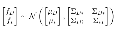
Suppose we have multivariate Gaussian Distribution below (5), and already got N samples from this Gaussian Process. And What we are going to gain is posterior distribution given f_N=y (6).

\begin{align}
\begin{bmatrix}
f_N \\
f_{*}
\end{bmatrix}
\sim \mathcal{N} \left(
\begin{bmatrix}
\mu_N \\
\mu_{*}
\end{bmatrix},
\begin{bmatrix}
\Sigma_{NN} & \Sigma_{N*} \\
\Sigma_{*N} & \Sigma_{**}
\end{bmatrix}
\right)\\
\mathcal{N}(\mu_{*|y}, \Sigma_{*|y} | f_N=y)\\
\end{align}

It turns out that estimate mean \mu_{*|y} and Variance\Sigma_{*|y}given y. The mean and covariance of a general conditional normal distribution are as follows;

\begin{align}
\mu_{*|Y} = \mu_* + \Sigma_{*N} \Sigma_{NN}^{-1} (y - \mu_N)\\
\Sigma_{*|Y} = \Sigma_{**} - \Sigma_{*N} \Sigma_{NN}^{-1} \Sigma_{N*}
\end{align}

Using these general conditional probability formulas, the mean and variance at a new sampling point (x*) can be calculated. When prior mean is zero vector,

\begin{align}
\mu_N(x_*) = k_N(x_*)^T \Sigma_{NN}^{-1} y\\
\sigma_N^2(x_*) = k(x_*, x_*) - k_N(x_*)^T \Sigma_{NN}^{-1} k_N(x_*)\\
k_N(x)=(k(x_*,x_1),k(x_*,x_2),,,k(x_*,x_N))^T\\
\end{align}

and when we introduce additive Gaussian noise, it just adds \sigma^2I_N.

\Sigma_{NN}^{update}=\Sigma_{NN} + \sigma^2I_N

The advantage of using the Gaussian process is that it is very easy to introduce posterior distribution like this since it is Gaussian, but it has complexity and flexibility since the kernel matrix is used in covariance matrix.