About
High-Dimensional Bayesian Optimization with Sparse Axis-Aligned Subspaces, so called SAASBO (https://arxiv.org/abs/2103.00349) uses Log Normal distribution and Half-Cauchy Distribution on its modeling. Since it is used as prior knowledge, it is good to know.
Log Normal Distribution
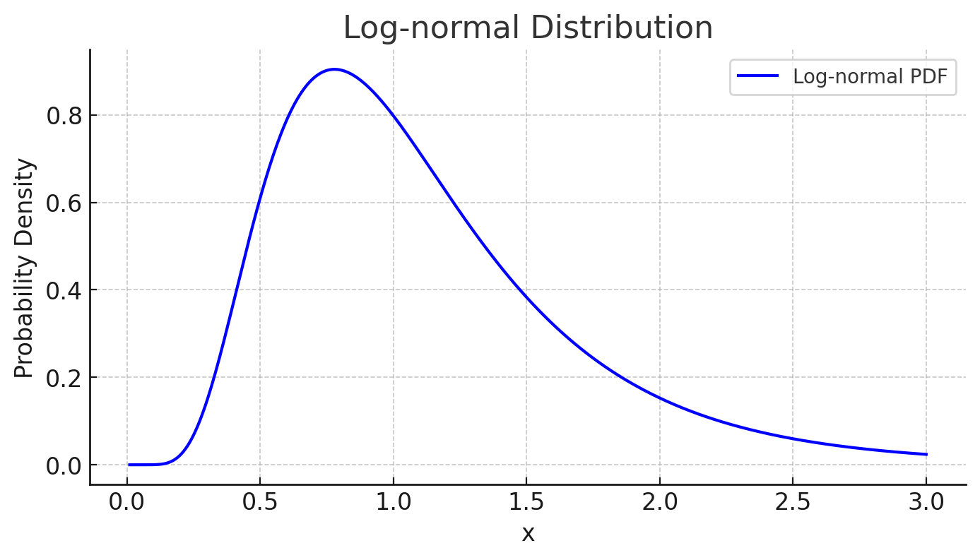
Log-normal distribution refers to the distribution of a random variable (X) when its natural logarithm (\ln(X)) follows a normal distribution. Specifically, if (\ln(X)) follows a normal distribution (N(\mu, \sigma^2)) with mean (\mu) and standard deviation (\sigma), then (X) follows a log-normal distribution. The probability density which is derived from normal distribution is written as follows
f_Z(z) = \frac{1}{\sqrt{2\pi} \sigma} \exp\left(-\frac{(z-\mu)^2}{2\sigma^2}\right)\\
f_X(x) = f_Z(\ln(x)) \left| \frac{d}{dx}\ln(x) \right|=f_Z(\ln(x)) \cdot \frac{1}{x}\\
=\frac{1}{x} \frac{1}{\sqrt{2\pi} \sigma} \exp\left(-\frac{(\ln(x) - \mu)^2}{2\sigma^2}\right)
The probability density function of the log-normal distribution is expressed as follows:
f(x) = \frac{1}{x\sigma\sqrt{2\pi}} e^{-\frac{(\ln x - \mu)^2}{2\sigma^2}} \quad \text{for } x > 0
Here,
- ( x ) is the value of ( X ) and ( x > 0 )
- ( \mu ) and ( \sigma ) are the mean and standard deviation of ( \ln(X) ), respectively.
The log-normal distribution is often found in nature and economic activities where positive, asymmetric distributions are observed. Typical examples include the distribution of income, stock returns, and city population. The distribution is characterized by a median smaller than the mean and a long right tail.

In the lognormal distribution, ( \mu = 0 ) means that the mean of the natural logarithm of ( X ), ( \ln(X) ), is 0. However, the distribution of ( X ) itself is based on the values before taking the logarithm, so its mean does not directly correspond to ( \mu ).
The median of the lognormal distribution is ( e^\mu ), where ( e^0 = 1 ). However, the shape of the distribution is asymmetric, with the mean being ( \text{exp}(\mu + \sigma^2 / 2) ), so the “center” of the distribution shifts. In particular, the larger the value of ( \sigma ), the more asymmetric the shape of the distribution becomes, and the further the mean shifts to the right.
To briefly summarize, the log-normal distribution is as follows:
\begin{align}
\text{ Median }(X) =  e^\mu \\
\text{ Mean}(X) =  e^{\mu + \sigma^2 / 2}\\
\text{Var}(X) = (e^{\sigma^2} - 1) e^{2\mu + \sigma^2}
\end{align}
The distribution is asymmetric, especially with a long tail on the right
Use Case?
This distribution is useful when data only have positive values, contains natural growth processes or multiplicative noise, or have very high values.
(Half-)Cauchy Distribution
The half-Cauchy distribution is a probability distribution derived from the Cauchy distribution, and is primarily applicable to positive real-valued data. The half-Cauchy distribution is an asymmetric version of the original Cauchy distribution, and in particular its probability density function is defined in the domain ( x \geq 0 ).
The probability density function of the Cauchy distribution is defined as:
f(x) = \frac{1}{\pi} \frac{\gamma}{(x - x_0)^2 + \gamma^2}The probability density function of the half-Cauchy distribution is the positive part of the Cauchy distribution, properly normalized. The probability density function for the location parameter (x_0) = 0 and the range (x\geq 0) is:
f(x) = \frac{2}{\pi} \frac{\gamma}{x^2 + \gamma^2}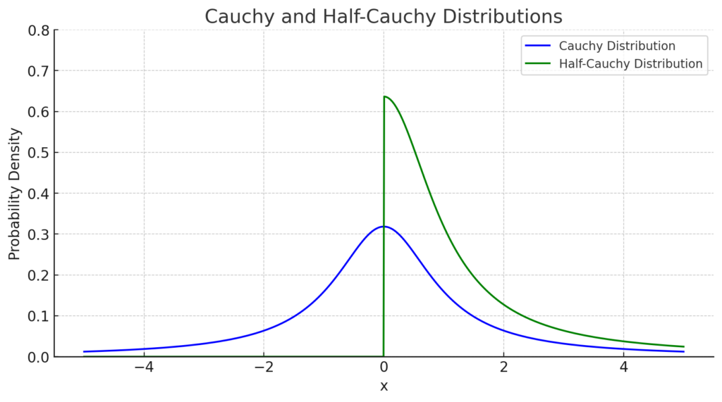
A characteristic feature of the Cauchy and Half-Cauchy distribution is that it has no mean or variance.
Use Case?
The Half-Cauchy distribution is particularly well suited for financial risk and insurance claims analysis, as it is robust to outliers and data where extreme values are common. It is also used as a prior distribution in Bayesian statistics, where it is useful for modeling variance parameters and other positively constrained parameters. The distribution is characterized by non-informativeness and heavy tails.