Bottleneck of computing Exact Gaussian Process
Suppose we have n-dimensional Gaussian Process below which consist of n number of data.
\begin{align}
f_n
\sim \mathcal{N} \left(
\mu_n,
\Sigma_{nn}\right)
\end{align}
To represent this distribution, n-dimensional covariance matrix is used.
\Sigma_{nn} = \begin{pmatrix}
k(\mathbf{x}_1, \mathbf{x}_1) & \cdots & k(\mathbf{x}_1, \mathbf{x}_N) \\
\vdots & \ddots & \vdots \\
k(\mathbf{x}_N, \mathbf{x}_1) & \cdots & k(\mathbf{x}_N, \mathbf{x}_N)
\end{pmatrix}
And to infer posterior distribution, the inverted covariance matrix should be computed.
\begin{align}
\mu_{*|Y} = \mu_* + \Sigma_{*n} \Sigma_{nn}^{-1} (f_n - \mu_n)\\
\Sigma_{*|Y} = \Sigma_{**} - \Sigma_{*n} \Sigma_{nn}^{-1} \Sigma_{n*}
\end{align}
Since the Exact GP uses n-number of data as it is for representing distribution, this computation can be bottleneck in big data era. For example, this algorithm has a computational complexity of \mathcal{O}(n^3), \mathcal{O}(n^2) of memory is needed. This things is what inducing points is going to solve.
Inducing Points and its purpose
The basic idea is to approximate the entire dataset using a small number of points, called inducing points, m. If m is much smaller than the total number of data points n, the computational burden can be significantly reduced.
Both the inducing point method and the Variational Gaussian process are fundamentally represented by the following probabilistic model. In this sense, the two are quite similar.
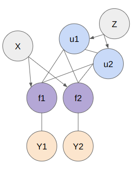
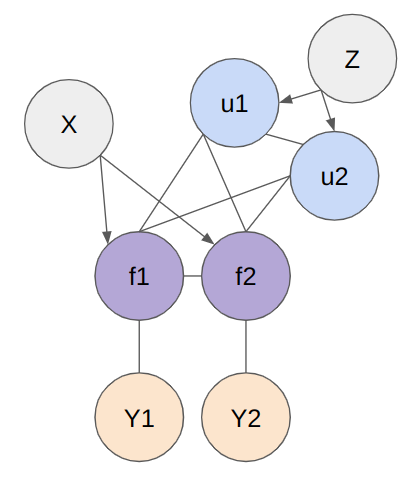
Below figure shows the structure of model. The X represents the entire set of data points, f is the random variable representing the entire dataset, Z denotes the inducing points, u represents the probability distribution over the inducing points, and Y is the random variable of the target function derived from the explanatory variable f . To represent the model, basically 2 models (SoR and FITC) are used.
Subset of Regressors (SoR)
The purpose of this method (which is so called SoR) is to apporximate gram matrix K_{nn} with K_{nm} K_{mm}^{-1} K_{mn}. To consider the approximation, joint probability of \mathbf{f}, \mathbf{u} is introduced.
\begin{bmatrix}
\mathbf{f} \\
\mathbf{u}
\end{bmatrix}
\sim \mathcal{N}\left(
\mathbf{0},
\begin{bmatrix}
\mathbf{K}_{nn} & \mathbf{K}_{nm} \\
\mathbf{K}_{mn} & \mathbf{K}_{mm}
\end{bmatrix}
\right)\\
Since the probability of both f and u are Gaussian distribution, the probability of f given u is explicitly written as follows
\begin{align}
f \mid u \sim \mathcal{N}\left(\mathbf{K}_{nm} \mathbf{K}_{mm}^{-1} \mathbf{u}, \mathbf{K}_{nn} - \mathbf{K}_{nm} \mathbf{K}_{mm}^{-1} \mathbf{K}_{mn}\right)
\end{align}
This is a simple method with induction points, but has low approximation accuracy.
Fully Independent Training Conditional(FITC)
The Fully Independent Training Conditional(FITC) improves on SoR by providing an approximation that takes into account the conditional dependencies between observations. The FITC approximates K_{nn} as follows
K_{nn} \approx
\underbrace{Q_{nn}}_{\text{Low-rank approximation via inducing points}}
+
\underbrace{\text{diag}(K_{nn} - Q_{nn})}_{\text{Independent variance of non-inducing observations}}.\\
\text{where} \space \mathbf{Q}_{nn} = \mathbf{K}_{nm} \mathbf{K}_{mm}^{-1} \mathbf{K}_{mn}.
As you can see in the covariance matrix, It is represented by the first term, which is a low-rank approximation via inducing points, and the second term, which accounts for the independent variance of non-inducing observations. Anyway, prior distribution of f is
f \sim \mathcal{N}(\mathbf{0}, \mathbf{Q}_{nn} + \text{diag}(\mathbf{K}_{nn} - \mathbf{Q}_{nn}))And the distribution of f given u is written as follows
\begin{align}
f \mid u \sim \mathcal{N}(\mathbf{K}_{nm} \mathbf{K}_{mm}^{-1} \mathbf{u}, \text{diag}(\mathbf{K}_{nn} - \mathbf{Q}_{nn}))
\end{align}
As you can see in (5), the covariance matrix of f given u becomes diagonal matrix.
But what does it indicate?
If we use \mathbf{Q}{nn} + \text{diag}(\mathbf{K}{nn} - \mathbf{Q}_{nn}) for \mathbf{K}_{NN}, the covariance simply becomes \text{diag}(\mathbf{K}{nn} - \mathbf{Q}_{nn}) which is diagonal matrix. It means that computation cost is low.

In practice, more complex models can be considered, but for simplicity, models without dependencies (uncorrelated) between f variables are often used.
Algorithms that utilize Inducing Points
KISS-GP is a method that uses a fixed grid structure of inducing points to efficiently approximate the kernel matrix. SKI extends KISS-GP by introducing more flexible interpolation techniques. SKIP further builds upon SKI to make it applicable to higher-dimensional data.
However, these methods are extensions of Exact Gaussian Processes (ExactGP) and do not fully eliminate the computational bottleneck. To address this, we introduce variational algorithms that, at first glance, resemble the modeling approach of inducing point methods.
The difference between Inducing Point Methods and Variational GP
The modeling of the two methods may seem the same, but what exactly is different?
Strictly speaking, the modeling is slightly different. In the inducing point method, the optimization target is essentially the inducing points themselves, not the distribution of the inducing points.
In variational Gaussian processes, in addition to this, the distribution q(u) of the inducing points u is also included as an optimization target. This q is used to learn an approximate distribution of the Gaussian process through variational inference.
q(u) = \mathcal{N}(m, S)A Gaussian distribution is also used for q . It seems that variational Gaussian processes offer a more flexible model compared to the inducing point method.
The inducing point method on the other hands, fixed prior distribution is used for u with kernel parameters(It highly depends on parameters in kernel, in contrast to variational approach).
p(u) = \mathcal{N}(0, \mathbf{K}_{mm})Modeling of Induction Point
In order to see how this approximation is conducted it in detail, I will write down detailed graphical model of a Gaussian process as follows.
\begin{align}
p(y | f) = \mathcal{N}\left( 0, \beta^{-1} \mathbf{I} \right)\\
p(f | u) = \mathcal{N}\left( f \mid \mathbf{K}_{nm} \mathbf{K}_{mm}^{-1} u, \mathbf{K}_{e} \right)\\
p(u) = \mathcal{N}(0, \mathbf{K}_{mm})\\
\end{align}
However, the important point is that this matrix K_{nn} in K_e is included in the model. It turns out that this computational complexity is high.
\mathbf{K}_e = \mathbf{K}_{nn} - \mathbf{K}_{nm} \mathbf{K}_{mm}^{-1} \mathbf{K}_{mn}In this paper[1], the correlation between n sampled points are removed so that K_{e} is diagonal as we showed above.
Optimization
So many methodologies of optimization are suggested, actually. for example,
\log p(y | u) = \log \mathbb{E}_{p(f | u)} \left[ p(y | f) \right]
\geq \mathbb{E}_{p(f | u)} \left[ \log p(y | f) \right] = \mathcal{L}_1
The paper[1] says that the more rough approximation you used, the faster computational complexity you get. But we should take care of fitting capability, which is the most important for Bayesian Optimization, to get quick convergence.
Reference
[1] James Hensman, Nicolo Fusi, Neil D. Lawrence “Gaussian Process for Big Data” https://arxiv.org/abs/1309.6835
[2] Andrew Gordon Wilson, Hannes Nickisch “Kernel Interpolation for Scalable Structured Gaussian Processes (KISS-GP)” https://arxiv.org/abs/1503.01057