Numeric and Categorical data handling

About

It is quite important to deal with both numeric and categorical data simultaneously when we get tabular dataset. But its data handling is sometimes annoying. I will summarize some of functions that I frequently used.

Load and filter data

It is common to read data with mixed categorical and numerical variables, as well as to delete rows with missing data when developing algorithms. Here, I will summarize those basic processes.

import pandas as pd

# データフレームの作成
data = pd.DataFrame({
    'Name': ['Alice', 'Bob', '', 'Charlie'],
    'Age': [25, 30, None, 22],
    'Gender': ['Female', 'Male', 'Male', ''],
    'Income': [50000, 60000, 45000, 70000]
})

# 列番号で列を選択
selected_columns = data.iloc[:, [0, 1, 2]]

# NaNの行を削除
filtered_data = selected_columns.dropna()

# 数値列とカテゴリ列を取得
numeric_columns = filtered_data.select_dtypes(include=['number'])
categorical_columns = filtered_data.select_dtypes(include=['object'])

# 数値列のインデックスを取得
numeric_column_indices = [data.columns.get_loc(col) for col in numeric_columns]

# カテゴリ変数をワンホットエンコーディング
encoded_categorical = pd.get_dummies(categorical_columns, drop_first=True)

# 数値列とエンコードされたカテゴリ列を結合
final_data = pd.concat([numeric_columns, encoded_categorical], axis=1)

# 結果を表示
print(final_data)

One Hot Encoding

In machine learning projects, you should use drop_first=True option in pd.get_dummies function. If it is True, it automatically removes first one hot categorical variable to avoid Multicollinearity. Let’s see how it works

import pandas as pd

# データの作成
data = pd.DataFrame({
    'Color': ['Red', 'Blue', 'Green', 'Blue', 'Red'],
    'Size': [10, 20, 30, 20, 10],
    'Price': [100, 150, 200, 130, 120]
})

# 'Color'列のワンホットエンコーディング
encoded_data = pd.get_dummies(data, columns=['Color'])

# 結果の表示
print(encoded_data)

this code exports following output.

   Size  Price  Color_Blue  Color_Green  Color_Red
0    10    100           0            0          1
1    20    150           1            0          0
2    30    200           0            1          0
3    20    130           1            0          0
4    10    120           0            0          1

But if you use the option = True, the result turns into like this, since there is redundant representation for machine learning.

   Size  Price  Color_Blue  Color_Green
0    10    100           0            0
1    20    150           1            0
2    30    200           0            1
3    20    130           1            0
4    10    120           0            0

Visualization

Visualizing data is one of the most important part of ml project. to visualize both numeric and categorical variables, following functions would be useful.

import pandas as pd
import numpy as np
import matplotlib.pyplot as plt
from pandas.api.types import is_categorical_dtype, is_object_dtype

def plot_with_color_axis(data, x_column, y_column):
    x = data[x_column]
    y = data[y_column]

    # 変数がカテゴリ型の場合、数値に変換
    if is_categorical_dtype(x) or is_object_dtype(x):
        x = pd.Categorical(x).codes
    if is_categorical_dtype(y) or is_object_dtype(y):
        y = pd.Categorical(y).codes

    # 図の作成
    plt.figure(figsize=(8, 6))
    scatter = plt.scatter(x, y, c=y, cmap='viridis')

    # カラーバーの作成
    plt.colorbar(scatter, label=f'{y_column} Categories')
    plt.title(f'Scatter plot of {x_column} vs {y_column}')
    plt.xlabel(x_column)
    plt.ylabel(y_column)

    plt.show()

# データの作成
data = pd.DataFrame({
    'Color': ['Red', 'Blue', 'Green', 'Blue', 'Red'],
    'Size': [10, 20, 30, 20, 10],
    'Price': [100, 150, 200, 130, 120]
})

# 関数の実行
plot_with_color_axis(data, 'Color', 'Size')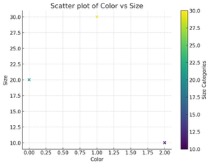

Compute joint probability

To take statistics, it’s important to compute joint probabilities

def calculate_probability(df, condition):
    return condition.sum() / len(df)

condition = (data['Gender'] == 'Female') & (data['Income'] > 100000)
probability = calculate_probability(data, condition)

print(f"'Female' and 'Income > 100000'の確率: {probability}")

Reasoning

Ifyou use one hot encoding, the relation between original input and encoded vector get complicated. But most of the cases , we are interested in the reasoning of the ml models. It should be clarified where the encoded variable came from.

import pandas as pd
import numpy as np
from sklearn.ensemble import RandomForestClassifier
from sklearn.model_selection import train_test_split

# データの作成
data = pd.DataFrame({
    'Color': ['Red', 'Blue', 'Green', 'Blue', 'Red'],
    'Size': [10, 20, 30, 20, 10],
    'Price': [100, 150, 200, 130, 120],
    'Target': [0, 1, 0, 1, 0]  # 目的変数の設定
})

# カテゴリ変数のエンコード（drop_first=True）
encoded_data_drop_first = pd.get_dummies(data, columns=['Color'], drop_first=True)

# 特徴量と目的変数に分割
X_drop_first = encoded_data_drop_first.drop('Target', axis=1)
y = encoded_data_drop_first['Target']

# トレーニングデータとテストデータに分割
X_train, X_test, y_train, y_test = train_test_split(X_drop_first, y, test_size=0.3, random_state=42)

# モデルの作成
model = RandomForestClassifier()
model.fit(X_train, y_train)

# 推論
predictions = model.predict(X_test)

# 特徴量の重要度
feature_importances = model.feature_importances_

importance_df = pd.DataFrame({'Feature': X_drop_first.columns, 'Importance': feature_importances})
importance_df = importance_df.sort_values(by='Importance', ascending=False)