Gridap-vs-Ngsolve-vs-Skfem

About

In the past, I compared computational cost between Skfem(Scikit-fem) and Ngsolve. Without doing experiments, I had already known the superiority of Ngsolve in terms this point, but I was unsure how much difference there is between them. What I found is that Scikit-fem is not so compettive with Ngsolve, but not super bad.

But I felt like, I want to have other option for solving heavier tasks. For sure we can use Ngsolve, but C++ language is NOT user friendly. Even though we have Python interface to access Ngsolve, the flexibility is limited.

To compare with other option, “Gridap” which I introduced before, I implemented script that solve FEM on the same task.

Result

This is what I really wanted😊

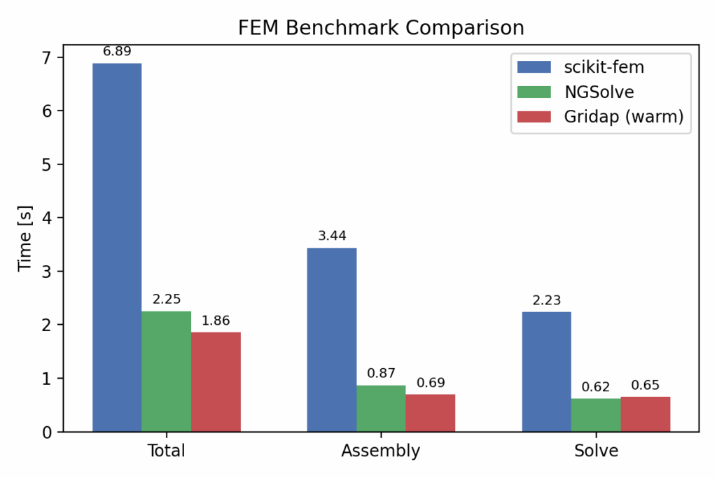
However, it should be noted that these results correspond to a warm start (i.e., the second and subsequent runs). During the first execution, JIT compilation is performed, which consumes computational resources in addition to the actual numerical calculation. As a result, the first run takes a total of 51.6 seconds, whereas subsequent runs are accelerated to under 2 seconds.

While Gridap already offers advantages such as convenient handling of I/O and integration with various packages, this study shows that it also delivers excellent computational performance.

In addition, I had forgotten to mention that Gridap also supports automatic differentiation.

Implementation

import time
import numpy as np
import skfem as sk


def run_skfem(mesh_file: str):
    from skfem.models.elasticity import lame_parameters
    from skfem.models.elasticity import linear_elasticity
    from skfem.helpers import dot

    E, nu = 210e3, 0.3
    traction_value = 1e-3
    lam, mu = lame_parameters(E, nu)

    t0_total = time.perf_counter()
    mesh = sk.MeshTet.load(mesh_file)
    basis = sk.Basis(mesh, sk.ElementVector(sk.ElementTetP1()))
    print(f"mesh.p {mesh.p.shape}")

    # @sk.BilinearForm
    # def elasticity(u, v, w):
    #     eps_u, eps_v = sk.sym_grad(u), sk.sym_grad(v)
    #     return lam * sk.trace(eps_u) * sk.trace(eps_v) + 2 * mu * sk.ddot(eps_u, eps_v)

    @sk.LinearForm
    def traction(v, w):
        return traction_value * dot(np.array([1, 0, 0]), v)

    left = mesh.facets_satisfying(lambda x: np.isclose(x[0], 0))
    right = mesh.facets_satisfying(lambda x: np.isclose(x[0], 1.0))
    fixed = basis.get_dofs(facets=left).all()
    print(f"fixed:{fixed.shape}")
    fbasis = sk.FacetBasis(
        mesh, sk.ElementVector(sk.ElementTetP1()), facets=right
    )

    # アセンブリ
    t0 = time.perf_counter()
    # K = sk.asm(elasticity, basis)
    K = linear_elasticity(lam, mu).assemble(basis)
    F = sk.asm(traction, fbasis)
    t_asm = time.perf_counter() - t0

    # Dirichlet条件 + 解く
    K, F = sk.enforce(K, F, D=fixed)
    t1 = time.perf_counter()
    u = sk.solve(K, F)
    t_solve = time.perf_counter() - t1

    t_total = time.perf_counter() - t0_total

    print(f"[scikit-fem] Total: {t_total:.3f}s | Assembly: {t_asm:.3f}s | Solve: {t_solve:.3f}s | max|u|={np.abs(u).max():.3e}")
    return mesh.p.T, u.reshape(-1, 3), [t_total, t_asm, t_solve]


def run_ngsolve(mesh_file: str):
    import time
    import numpy as np
    from ngsolve import (
        Mesh, VectorH1, BilinearForm, LinearForm, GridFunction,
        CoefficientFunction, grad, Trace, Id, InnerProduct,
        dx, ds, x, IfPos,
    )
    from netgen.read_gmsh import ReadGmsh

    # --- 材料・荷重パラメータ ---
    E, nu = 210e3, 0.3
    traction_value = 1e-3
    lam = E * nu / ((1 + nu) * (1 - 2 * nu))
    mu = E / (2 * (1 + nu))

    t0_total = time.perf_counter()

    # --- メッシュ読み込み (.msh) ---
    ngmesh = ReadGmsh(mesh_file)
    mesh = Mesh(ngmesh)
    print(f"nv = {mesh.nv}")

    # --- x のレンジを自動取得 ---
    xs = [vtx.point[0] for vtx in mesh.vertices]
    xmin, xmax = min(xs), max(xs)
    print(f"x-range: [{xmin:.6g}, {xmax:.6g}]")

    # Dirichlet は座標で後から指定するので、ここでは dirichlet="" は指定しない
    fes = VectorH1(mesh, order=1)

    u = fes.TrialFunction()
    v = fes.TestFunction()

    # --- 線形弾性の弱形式 ---
    def eps(w):
        return 0.5 * (grad(w) + grad(w).trans)

    def sigma(w):
        return lam * Trace(eps(w)) * Id(3) + 2 * mu * eps(w)

    a = BilinearForm(fes, symmetric=True)
    a += InnerProduct(sigma(u), grad(v)) * dx

    # --- Neumann: x ≈ xmax の面だけに traction をかける ---
    eps_coord = 1e-8 * max(1.0, abs(xmax - xmin))  # スケールに合わせて少しだけ幅を取る
    # x > xmax - eps のとき 1、それ以外 0
    indicator_right = IfPos(x - (xmax - eps_coord), 1.0, 0.0)

    tvec = CoefficientFunction((traction_value, 0.0, 0.0))
    f = LinearForm(fes)
    # 「すべての境界 ds」に対して、x≃xmax のところだけ traction が効く
    f += InnerProduct(indicator_right * tvec, v) * ds

    # --- アセンブリ ---
    t0 = time.perf_counter()
    a.Assemble()
    f.Assemble()
    t_asm = time.perf_counter() - t0

    print("||f|| =", f.vec.Norm())  # 荷重がちゃんと入っているか確認用

    # --- GridFunction と FreeDofs（BitArray コピー） ---
    gfu = GridFunction(fes)

    freedofs0 = fes.FreeDofs()             # BitArray
    freedofs = type(freedofs0)(freedofs0)  # 古い NGSolve 向けコピー

    # --- Dirichlet: x ≈ xmin の頂点の DoF を拘束 & 0 固定 ---
    for vtx in mesh.vertices:
        if abs(vtx.point[0] - xmin) < eps_coord:
            dnums = fes.GetDofNrs(vtx)  # この頂点に対応する DoF 番号
            for d in dnums:
                freedofs[d] = False   # 拘束
                gfu.vec[d] = 0.0      # Dirichlet 値

    # --- 解く ---
    t1 = time.perf_counter()
    gfu.vec.data = a.mat.Inverse(freedofs, inverse="sparsecholesky") * f.vec
    t_solve = time.perf_counter() - t1

    t_total = time.perf_counter() - t0_total

    # --- 頂点座標と変位を numpy 配列に ---
    coords = np.zeros((mesh.nv, 3))
    u_vals = np.zeros((mesh.nv, 3))

    for i, vtx in enumerate(mesh.vertices):
        p = vtx.point
        x0, y0, z0 = p[0], p[1], p[2]
        coords[i, :] = (x0, y0, z0)

        # MeshPoint を通して点評価
        val = gfu(mesh(x0, y0, z0))
        u_vals[i, :] = np.array(val)

    print(
        f"[NGSolve] Total: {t_total:.3f}s | "
        f"Assembly: {t_asm:.3f}s | "
        f"Solve: {t_solve:.3f}s | "
        f"max|u|={np.max(np.abs(u_vals)):.3e}"
    )

    return coords, u_vals, [t_total, t_asm, t_solve]


def visualize(
    skfem_times, ngsolve_times,
    dst_path: str = "benchmark_comparison.jpg"
):
    import matplotlib.pyplot as plt
    import numpy as np

    # データ（あなたの測定結果）
    labels = ["Total", "Assembly", "Solve"]
    
    x = np.arange(len(labels))  # X軸位置
    width = 0.35                # 棒の幅

    fig, ax = plt.subplots(figsize=(6, 4))
    rects1 = ax.bar(x - width/2, skfem_times, width, label='scikit-fem', color='#4C72B0')
    rects2 = ax.bar(x + width/2, ngsolve_times, width, label='ngsolve', color='#55A868')

    # 軸ラベル・タイトル
    ax.set_ylabel('Time [s]')
    ax.set_title('FEM Benchmark Comparison')
    ax.set_xticks(x)
    ax.set_xticklabels(labels)
    ax.legend()

    # 各棒に値を表示
    def autolabel(rects):
        for rect in rects:
            height = rect.get_height()
            ax.annotate(f'{height:.2f}',
                        xy=(rect.get_x() + rect.get_width() / 2, height),
                        xytext=(0, 3),
                        textcoords="offset points",
                        ha='center', va='bottom', fontsize=9)

    autolabel(rects1)
    autolabel(rects2)

    fig.tight_layout()
    plt.savefig(dst_path, dpi=200)
    # plt.show()

    print("✅ Saved: benchmark_comparison.png")


def compare_displacements(coords1, u1, coords2, u2, tol=1e-8):
    # 両メッシュが一致する前提
    assert np.allclose(coords1, coords2, atol=tol)

    diff = u1 - u2
    abs_err = np.linalg.norm(diff, axis=1)
    l2_err = np.linalg.norm(abs_err)
    rel_err = l2_err / np.linalg.norm(np.linalg.norm(u1, axis=1))
    max_err = np.max(abs_err)

    print(f"‣ L2 error = {l2_err:.3e}")
    print(f"‣ Relative L2 error = {rel_err:.3e}")
    print(f"‣ Max abs error = {max_err:.3e}")


if __name__ == "__main__":
    msh = "tension_bar.msh"  # Gmshで生成済みメッシュ

    print("run_skfem")
    skfem_coords, skfem_disp, skfem_times = run_skfem(msh)

    print("run_ngsolve")
    ngsolve_coords, ngsolve_disp, ngsolve_times = run_ngsolve(msh)
    tT_s, tA_s, tS_s = skfem_times
    tT_m, tA_m, tS_m = ngsolve_times

    print("skfem max|u| =", np.abs(skfem_disp).max())
    print("ngsolve  max|u| =", np.abs(ngsolve_disp).max())
    print("ratio (skfem/ngsolve) ≈", np.abs(skfem_disp).max() / np.abs(ngsolve_disp).max())

    compare_displacements(skfem_coords, skfem_disp, ngsolve_coords, ngsolve_disp)

    print("\n=== Benchmark Summary ===")
    print(f"scikit-fem: Total {tT_s:.3f}s | Assembly {tA_s:.3f}s | Solve {tS_s:.3f}s")
    print(f"ngsolve:       Total {tT_m:.3f}s | Assembly {tA_m:.3f}s | Solve {tS_m:.3f}s")

    visualize(
        skfem_times, ngsolve_times,
    )

Result