Physics Informed Neural Network

https://arxiv.org/abs/1711.10561

I found an interesting thesis, ”Physics Informed Deep Learning: Data-driven Solutions of Nonlinear Partial Differential Equations. Generally, Partial differential equations(PDE) are solved by using matrix manipulations like FEM, but this way is using Deep Neural Network as PDE solver.

One of the interesting things about Deep Neural Network is that it enables us to get gradients(derivatives) of parameters. We can also obtain the second-order and higher derivatives of parameters from Deep Neural Networks.

The key idea for a Deep Neural Network PDE solver is to optimize Deep Neural Network parameters so that satisfying Partial differential equations and boundary conditions. Therefore obtaining derivatives from Networks enables us to optimize those parameters, and we can define the loss functions that optimize loss functions for PDE and boundary conditions.

There are mainly 2 approaches for Physics Informed Neural Networks (PINN), Continuous Time Models and Discrete Time Models.

Continuous Time Models

The model is going to deal with all parameters (like time, spacial parameters x, y, and z) on equations as same. It means that if we feed the parameters t(time) and x, the Neural Network returns the field values.

\begin{align} f_1(t, x) = u\\ f_2(t, x) = v\\ \end{align}

I represent derivatives like (3)-(5).

\begin{align} \frac{df_1(t, x)}{dt} = u_t\\ \frac{df_1(t, x)}{dt} = u_x\\ \frac{d^2f_1(t, x)}{dt^2} = u_{xx}\\ \end{align}

By using this Neural Network, we can define partial equation (6) and boundary conditions(7), (8).

\begin{align} u_t + uu_x + u_xx = 0\\ u(0, x) = Q(x)\\ u(t, 0) = 0 \end{align}

In the case of the burgers equation which has a closed-form solution and is often used for comparing with the predicted solution, PDE and BC are described below.

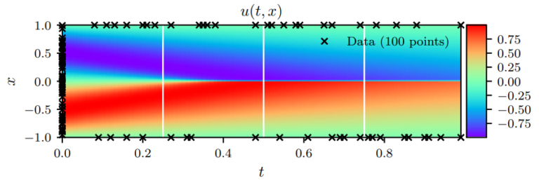
\begin{align} u_t + uu_x - \frac{0.01}{ \pi} u_xx = 0, x \in [-1, 1], t \in [-1, 1] \\ u(0, x) = -sin(\pi x),\\ u(t, -1) = u(t, 1) = 0 \end{align}

By optimizing (9)-(10) via MSE(mean root squared error), we get the PDE solution shown in Figure 1.

The x’ sign in Figure 1 shows the points that are used for optimizing boundary conditions. Regardless of the few data points (100 points) on the boundary, the solution looks absolutely wonderful.

Discrete Time Models

The other model is called the ‘Discrete Time Model’. Unlike Continuous Models, the Discrete Time Models do not deal with time and spacial variables (X, Y, and Z). The Discrete Time Models literally have field values each time (That is why it is called ‘Discrete’). But how do the models deal with time-wise differential equations? The model is using high-order Runge-Kutta methods to represent time transition (differential equation). This corresponds to the Neural Networks for Discrete-Time models having multiple outputs. The number of neural network outputs corresponds to the number of Runge-Kutta coefficients.

\begin{align} N(x) = [u_1, u_2,,,u_{q+1}] \end{align}

The models set loss function for time-wise differential equation by using Runge-Kutta coefficients. This gets to be a new loss function for the models.

\begin{align} u^{n+c_i}=u^n-\varDelta{t}\textstyle\sum_{j=1}^qa_{ij}\natnums[u^{n+c_j}] \quad i=1,,,q\\ u^{n+1}=u^n-\varDelta{t}\textstyle\sum_{j=1}^qb_{j}\natnums[u^{n+c_j}] \\ Where \quad u^{n+c_i}(x)=u(t^n+c_j\varDelta{t}, x) \end{align}

Actually, resemble methods that are using polynomial functions are already developed. But it is said that it is difficult to handle complex shapes. I am paying attention to if neural networks can solve this challenge.