The Concept of Optimal Transport

Why Optimal Transport?

Cross-Entropy: This is a measure used to quantify the difference between two probability distributions. Specifically, it’s used to evaluate the difference between the actual probability distribution (typically the distribution of the ground truth data) and the predicted probability distribution (predictions made by the model).

Binary Cross-Entropy: This is a special case of cross-entropy, used to measure the difference between two probability distributions that only have two categories (e.g., 0 and 1). It is primarily used in binary classification problems.

However, in cases where these metrics alone may not describe the phenomena well, optimal transport comes into play. The concept of optimal transport aims to minimize the “cost” when “transforming” from one distribution to another. Specifically, it seeks the most efficient way to move one probability distribution to another within a certain space. This concept is used from a perspective different from cross-entropy as another method to measure differences between distributions. The theory of optimal transport can capture differences in the shape and location of distributions more intuitively, making it very useful for certain applications.

The details of the differences will be discussed below.

The difference between Ground-Truth and Prediction

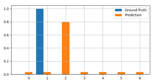
Suppose we have 2 distribution, Ground Truth and a Prediction from model. And the difference of the distribution between 2 is like Figure 1. In this case, your prediction from model is quite bad since It looks not close to the Ground Truth distribution. Not to get bad model like this, what sort of loss function should we introduce? For sure, this depends on the task.

Cross Entropy – Binary Cross Entropy

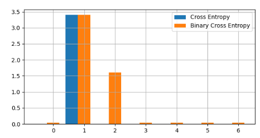
Here, both cross-entropy and binary cross-entropy are computed for each element of a distribution, as shown in Figure 2. So, what distinguishes the two? Cross entropy measures the difference between two probability distributions and is typically used for multi-class classification problems. The term “cross” in “cross-entropy” signifies that it compares two distributions. On the other hand, binary cross-entropy is a special case of cross entropy used specifically for binary classification problems. Each element is treated as an independent distribution over the binary labels, 0 or 1. The Figure 2 shows the distribution of Cross Entropy (Blue) and Binary Cross Entropy(Orange). As you can see, Binary Cross Entropy distriubution(Orange) is widely spread since Binary Cross Entropy takes both 0 and 1 labels into account.

Are you guys happy with just 2 loss function, Cross Entropy and Binary Cross Entropy?

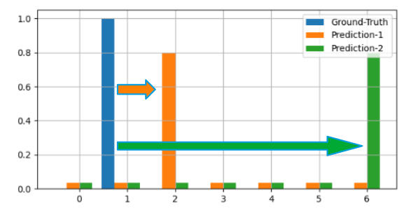
No absolutely Not. Think that below case, Figure 3.

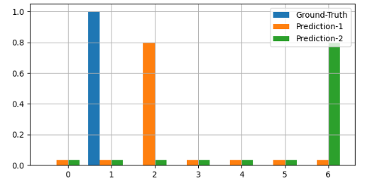
We have three distributions: Ground-Truth (Blue), Prediction-1 (Orange), and Prediction-2 (Green). Both Prediction-1 and Prediction-2 have the same peak values. However, the location of the peak in Prediction-2 is much further from the peak of Ground-Truth than Prediction-1 is. If we consider these distributions as categorical, using cross-entropy poses no issue. But if we view them as continuous distributions, employing cross-entropy becomes problematic. Why is that?

If we treat these distributions as continuous, then the Ground Truth distribution should be closer to Prediction-1, given that their peaks are near each other. In contrast, the distance between Ground Truth and Prediction-2 would be more significant due to the substantial separation between their peaks.

Let’s examine the cross-entropy (and binary entropy) for each element as presented in Figure 4.

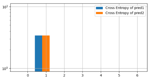
The Cross Entropy distribution of each prediction is shown as Blue and Orange Color. As you can see, each cross entropy It looks same. It means that the both loss values takes same value even if the difference(distance) of distribution from Ground Truth.

This is, the motivation of Optimal Transport Research. To consider situations where elements within two vectors that are close have significance, Optimal Transport might be useful.

What is the key idea of Optimal Transport?

The Key idea of Optimal Transport

The cross-entropy distributions for each prediction are represented in blue and green. As observed, both appear quite similar, implying that both loss values are the same, even if the differences (or distances) in their distributions from the Ground Truth vary.

This observation underscores the motivation behind Optimal Transport research. So, what’s the central concept of Optimal Transport?

How to define the loss functions of Optimal Transport?

There are multiple ways can be considered.

Let’s consider a simple one-dimensional vector. We’ll look at the following two vectors, p and q. Each represents a discrete probability distribution with n elements. When thinking about optimal transport, it’s necessary to define a transportation cost from one distribution to another. While there are various ways to do this, the Wasserstein distance (also known as the Earth Mover’s Distance, or EMD) seems to be a commonly mentioned cost function.