Optimization Solver : OpenMDAO

About

There are not many options for solving complex nonlinear optimization problems. When you want to try something out with open-source software, you might find yourself struggling to choose. Today, I came across a very promising project—OpenMDAO. It seems to provide solvers for constrained nonlinear optimization problems. Since it looked useful, I decided to give it a try. It would be useful for simulating physics phenomenon. It contains some solvers such as SLSQP or COBYLA, I do not touch how it solves the problem, but I will look into it in the future.

Optimization Problem

Objective

\min_{x}f(x) = \frac{1}{2} x^T Q x + c^T x \\
\text{subject to }Ax = b

Implementation

import numpy as np
import openmdao.api as om

class QuadraticObjective(om.ExplicitComponent):
    def initialize(self):
        self.options.declare('Q', types=np.ndarray)
        self.options.declare('c', types=np.ndarray)

    def setup(self):
        n = self.options['Q'].shape[0]
        self.add_input('x', shape=(n,))
        self.add_output('f', val=0.0)
        self.declare_partials('f', 'x')

    def compute(self, inputs, outputs):
        Q = self.options['Q']
        c = self.options['c']
        x = inputs['x']
        outputs['f'] = 0.5 * x @ Q @ x + c @ x

    def compute_partials(self, inputs, partials):
        Q = self.options['Q']
        c = self.options['c']
        x = inputs['x']
        partials['f', 'x'] = (Q @ x + c)

class LinearConstraint(om.ExplicitComponent):
    def initialize(self):
        self.options.declare('A', types=np.ndarray)
        self.options.declare('b', types=np.ndarray)

    def setup(self):
        A = self.options['A']
        m, n = A.shape
        self.add_input('x', shape=(n,))
        self.add_output('Ax_minus_b', shape=(m,))
        self.declare_partials('Ax_minus_b', 'x', val=A)

    def compute(self, inputs, outputs):
        A = self.options['A']
        b = self.options['b']
        x = inputs['x']
        outputs['Ax_minus_b'] = A @ x - b

# --- Define Q, c, A, b ---
Q = np.array([[2.0, 0.0], [0.0, 2.0]])
c = np.array([-4.0, -6.0])
A = np.array([[1.0, 1.0]]) 
b = np.array([1.0])

# --- Construct OpenMDAO Solver ---
prob = om.Problem()
model = prob.model

model.add_subsystem('objective', QuadraticObjective(Q=Q, c=c), promotes=['x', 'f'])
model.add_subsystem('constraint', LinearConstraint(A=A, b=b), promotes=['x', 'Ax_minus_b'])

model.add_design_var('x', lower=-10.0, upper=10.0)
model.add_objective('f')
# model.add_constraint('Ax_minus_b', lower=4.0, upper=0)
model.add_constraint('Ax_minus_b', equals=0.0)

prob.driver = om.ScipyOptimizeDriver(optimizer='SLSQP', tol=1e-6)

prob.setup()
prob.set_val('x', np.array([0.5, 0.5]))  # Initial Value
prob.run_driver()

# --- Result ---
print(f"Optimal x: {prob.get_val('x')}")
print(f"Optimal Objective: {prob.get_val('f')}")

Result

from matplotlib import pylab as plt

optimal_x = prob.get_val('x').flatten()
x_vals = np.linspace(-1, 2, 100)
y_vals = np.linspace(-1, 2, 100)
X, Y = np.meshgrid(x_vals, y_vals)
Z = 0.5 * (Q[0, 0] * X**2 + 2 * Q[0, 1] * X * Y + Q[1, 1] * Y**2) + c[0] * X + c[1] * Y

fig, ax = plt.subplots(figsize=(6, 6))

# 1. Quadrotic
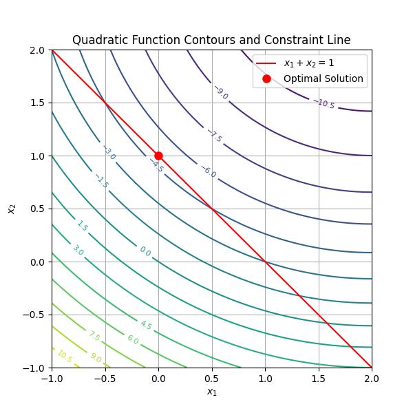
contours = ax.contour(X, Y, Z, levels=20, cmap="viridis")
ax.clabel(contours, inline=True, fontsize=8)

# 2. Ax = b 
x_line = np.linspace(-1, 2, 100)
y_line = 1 - x_line
ax.plot(x_line, y_line, 'r-', label=r'$x_1 + x_2 = 1$')

# 3.
ax.plot(optimal_x[0], optimal_x[1], 'ro', markersize=8, label="Optimal Solution")

ax.set_xlabel(r'$x_1$')
ax.set_ylabel(r'$x_2$')
ax.set_title("Quadratic Function Contours and Constraint Line")
ax.legend()
ax.grid(True)

plt.savefig("test.jpg")