Burgers Equation with Differential Physics, PhiFlow

Burgers Equation

The one-dimensional Burgers’ equation is expressed in the following formula

\frac{\partial u}{\partial t} + u \frac{\partial u}{\partial x} = \nu \frac{\partial^2 u}{\partial x^2}

Here, u represents the velocity field, t is time, and x is the spatial coordinate. The right-hand side of the equation contains the diffusion term, which is associated with fluid viscosity. The nonlinear advection term represents the role of the velocity field in transporting and deforming material. This equation describes the time and space evolution of the velocity field and is a nonlinear partial differential equation.

Key Idea

As we can see a chapter ‘differential physics’ in https://physicsbaseddeeplearning.org/diffphys.html, this solver is going to optimize solution using back propagation. So, what’s important is that write code of simulation using deeplearning framework in order to update solution via backprop.

Code

As we can see in an example of PD in https://physicsbaseddeeplearning.org/diffphys-code-burgers.html, key code is here. In order to use backprop,

# from phi import flow
from phi.tf import flow
# from phi.torch import flow

The loss function for optimization is following

def loss_function(velocity):
    velocities = [velocity]
    for time_step in range(STEPS):
        v1 = flow.diffuse.explicit(1.0*velocities[-1], NU, DT, substeps=1)
        v2 = flow.advect.semi_lagrangian(v1, v1, DT)
        velocities.append(v2)
    loss = flow.field.l2_loss(velocities[16] - SOLUTION_T16)*2./N # MSE
    return loss, velocities

Why is advection term estimated by diffusion term?

Since it is using Semi-Lagrangian method which High-order difference methods, are used. The Semi-Lagrangian method is an approach that utilizes high-order difference schemes and interpolation techniques when advecting materials according to the velocity field.

First-order difference methods provide relatively simple and coarse approximations in numerical computations, but they are insufficient for accurately modeling nonlinear advection equations. When it comes to simulating the movement of materials based on the velocity field, it is common to use higher-order difference methods. The Semi-Lagrangian method is one example of such advanced techniques, where it tracks the trajectories of materials using information from the velocity field and computes new material values through interpolation. This enables it to handle nonlinearity and irregular velocity fields.

Therefore, in the advect step, higher-order difference methods are employed rather than first-order difference methods. Using higher-order difference methods allows for a more accurate computation of material movement and deformation according to the velocity field.

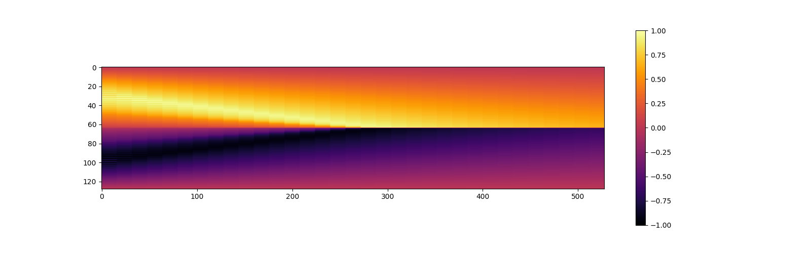
Result

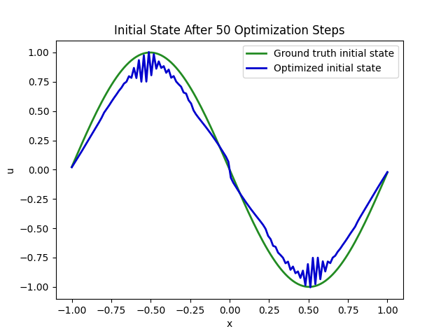
Although these results are as same result as example above, the solution is

The result looks quite fine, but actually not perfect as we can see below. The graph is comparison between ground truth and optimized solution at initial state.