Practice OpenMDAO

About

In the last article(https://eye.kohei-kevin.com/2025/03/03/optimization-solver-ooenmdao/), I tested simple non linear optimization problem with a liner constraint. I tried other form to practice implementing with OpenMDAO. I want to become familiar with this framework, gradually make the problems more complex, and develop them into interesting challenges.

Task

Objective

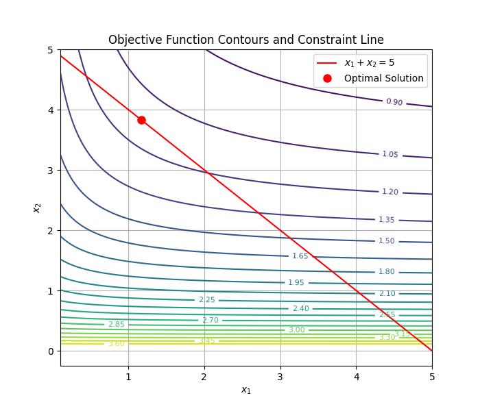
\min_{x}k^T X^{-1} k \\
\text{where }X = \begin{bmatrix} x_1 + 1 & 0.5 \\ 0.5 & x_2 + 1 \end{bmatrix}\\
\text{subject to } x_1+x_2=5

Result

Implementation

import numpy as np
import openmdao.api as om
from matplotlib import pylab as plt


class InverseQuadraticObjective(om.ExplicitComponent):
    """ minimize objective k^T X^{-1} k """

    def initialize(self):
        self.options.declare('k', types=np.ndarray)

    def setup(self):
        self.add_input('x', shape=(2,))
        self.add_output('f', val=0.0)
        self.declare_partials('f', 'x')

    def compute(self, inputs, outputs):
        x1, x2 = inputs['x']
        k = self.options['k']

        X = np.array([[x1 + 1, 0.5],
                      [0.5, x2 + 1]])

        X_inv = np.linalg.inv(X)

        outputs['f'] = k.T @ X_inv @ k

    def compute_partials(self, inputs, partials):
        x1, x2 = inputs['x']
        k = self.options['k']

        X = np.array([[x1 + 1, 0.5],
                      [0.5, x2 + 1]])

        X_inv = np.linalg.inv(X)

        dX1 = np.array([[1, 0], [0, 0]])
        dX2 = np.array([[0, 0], [0, 1]])

        dX1_inv = -X_inv @ dX1 @ X_inv
        dX2_inv = -X_inv @ dX2 @ X_inv

        partials['f', 'x'] = np.array([
            k.T @ dX1_inv @ k,
            k.T @ dX2_inv @ k
        ])

class LinearConstraint(om.ExplicitComponent):
    def setup(self):
        self.add_input('x', shape=(2,))
        self.add_output('g', val=0.0)
        self.declare_partials('g', 'x', val=[1.0, 1.0])

    def compute(self, inputs, outputs):
        x1, x2 = inputs['x']
        outputs['g'] = x1 + x2 - 5 


prob = om.Problem()
model = prob.model

k = np.array([1.0, 2.0])

model.add_subsystem('objective', InverseQuadraticObjective(k=k), promotes=['x', 'f'])
model.add_subsystem('constraint', LinearConstraint(), promotes=['x', 'g'])

model.add_design_var('x', lower=0.1, upper=5.0)
model.add_objective('f')
model.add_constraint('g', equals=0.0)

prob.driver = om.ScipyOptimizeDriver(optimizer='SLSQP', tol=1e-6)

prob.setup()
prob.set_val('x', np.array([0.5, 0.5]))
prob.run_driver()

optimal_x = prob.get_val('x')
optimal_f = prob.get_val('f')

x1_vals = np.linspace(0.1, 5.0, 100)
x2_vals = np.linspace(0.1, 5.0, 100)
X1, X2 = np.meshgrid(x1_vals, x2_vals)
Z = np.zeros_like(X1)

for i in range(X1.shape[0]):
    for j in range(X1.shape[1]):
        x1, x2 = X1[i, j], X2[i, j]
        X = np.array([[x1 + 1, 0.5], [0.5, x2 + 1]])
        X_inv = np.linalg.inv(X)
        Z[i, j] = k.T @ X_inv @ k

fig, ax = plt.subplots(figsize=(7, 6))

contours = ax.contour(X1, X2, Z, levels=20, cmap="viridis")
ax.clabel(contours, inline=True, fontsize=8)

x1_line = np.linspace(0.1, 5.0, 100)
x2_line = 5 - x1_line
ax.plot(x1_line, x2_line, 'r-', label=r'$x_1 + x_2 = 5$')

ax.plot(optimal_x[0], optimal_x[1], 'ro', markersize=8, label="Optimal Solution")

ax.set_xlabel(r'$x_1$')
ax.set_ylabel(r'$x_2$')
ax.set_title("Objective Function Contours and Constraint Line")
ax.legend()
ax.grid(True)

plt.savefig("test-2.jpg")